Light and Matter Fullerton, California www.lightandmatter.com
copyright 2005 Benjamin Crowell
rev. April 27, 2007
5
1 Rates of Change
1.1 Change in discrete steps 9Two sides of the same coin, 9.—Some guesses, 11.
1.2 Continuous change . . 12 A derivative, 14.—Properties of the derivative, 15.— Higher-order polynomials, 16.—The second derivative, 16.—Maxima and minima, 18.
Problems. . . 21
2 To infinity — and
beyond!
2.1 Infinitesimals. . . 23 2.2 Safe use of infinitesimals 26 2.3 The product rule . . . 30 2.4 The chain rule . . . . 33
2.5 Exponentials and
logarithms . . . 34 The exponential, 34.—The logarithm, 35.
2.6 Quotients . . . 36 2.7 Differentiation on a computer . . . 38 2.8 Continuity . . . 41 2.9 Limits . . . 41
L’Hˆopital’s rule, 42.— Another perspective on in-determinate forms, 44.
Problems. . . 46
3 Integration
3.1 Definite and indefinite integrals . . . 51 3.2 The fundamental theorem of calculus . . . 54 3.3 Properties of the integral 55 3.4 Applications . . . 56
Averages, 56.—Work, 57.—
Probability, 57.
Problems. . . 63
4 Techniques
4.1 Newton’s method . . . 65 4.2 Implicit differentiation . 66 4.3 Taylor series . . . 67 4.4 Methods of integration . 72
Change of variable, 72.— Integration by parts, 74.— Partial fractions, 75.
Problems. . . 79
5 Complex number
techniques
5.1 Review of complex numbers . . . 81 5.2 Euler’s formula . . . . 84 5.3 Partial fractions revisited 86 Problems. . . 87
6 Improper integrals
6.1 Integrating a function that blows up . . . 89 6.2 Limits of integration at infinity . . . 90 Problems. . . 927 Iterated integrals
7.1 Integrals inside integrals 93 7.2 Applications . . . 95 7.3 Polar coordinates . . . 97 7.4 Spherical and cylindrical coordinates . . . 98 Problems. . . 100B Answers and solutions
111C Photo Credits
129D Reference
131D.1 Review . . . 131 Algebra, 131.—Geometry,
area, and volume, 131.— Trigonometry with a right triangle, 131.—Trigonometry with any triangle, 131.
D.2 Hyperbolic functions . . 131 D.3 Calculus . . . 132
7
Preface
Calculus isn’t a hard subject. Algebra is hard. I still remem-ber my encounter with algebra. It was my first taste of abstraction in mathematics, and it gave me quite a few black eyes and bloody noses. Geometry is hard. For most peo-ple, geometry is the first time they have to do proofs using formal, ax-iomatic reasoning.
I teach physics for a living. Physics is hard. There’s a reason that peo-ple believed Aristotle’s bogus ver-sion of physics for centuries: it’s because the real laws of physics are counterintuitive.
Calculus, on the other hand, is a very straightforward subject that rewards intuition, and can be eas-ily visualized. Silvanus Thompson, author of one of the most popular calculus texts ever written, opined that “considering how many fools can calculate, it is surprising that it should be thought either a diffi-cult or a tedious task for any other fool to master the same tricks.” Since I don’t teach calculus, I can’t require anyone to read this book. For that reason, I’ve written it so that you can go through it and get to the dessert course with-out having to eat too many Brus-sels sprouts and Lima beans along the way. The development of any mathematical subject involves a large number of boring details that have little to do with the main
1 Rates of Change
1.1
Change in
discrete steps
Toward the end of the eighteenth century, a German elementary school teacher decided to keep his pupils busy by assigning them a long, boring arithmetic problem. To oversimplify a little bit (which is what textbook authors always do when they tell you about his-tory), I’ll say that the assignment was to add up all the numbers from one to a hundred. The chil-dren set to work on their slates, and the teacher lit his pipe, con-fident of a long break. But al-most immediately, a boy named Carl Friedrich Gauss brought up his answer: 5,050.
a/Adding the numbers from 1 to 7.
Figure a suggests one way of solv-ing this type of problem. The filled-in columns of the graph rep-resent the numbers from 1 to 7, and adding them up means
find-b/A trick for finding the sum.
ing the area of the shaded region. Roughly half the square is shaded in, so if we want only an approxi-mate solution, we can simply cal-culate 72/2 = 24.5.
But, as suggested in figure b, it’s not much more work to get an ex-act result. There are seven saw-teeth sticking out out above the di-agonal, with a total area of 7/2, so the total shaded area is (72 + 7)/2 = 28. In general, the sum of the first n numbers will be (n2+
n)/2, which explains Gauss’s re-sult: (1002+ 100)/2 = 5, 050.
Two sides of the same coin
c/Carl Friedrich Gauss (1777-1855), a long time after graduating from ele-mentary school.
Let’s label the years as n = 1, 2, 3,. . ., and let the function1 x(n) represent the amount of garbage that has accumulated by the end of year n. If the population is constant, say 13 households, then garbage accumulates at a constant rate, and we havex(n) = 13n. But maybe the town’s population is growing. If the population starts out as 1 household in year 1, and then grows to 2 in year 2, and so on, then we have the same kind of problem that the young Gauss solved. After 100 years, the accu-mulated amount of garbage will be 5,050 tons. The pile of refuse grows more and more every year; the rate of change ofxis not constant. Tab-ulating the examples we’ve done so far, we have this:
1Recall that whenxis a function, the
notation x(n) means the output of the function when the input isn. It doesn’t represent multiplication of a numberxby a numbern.
rate of change accumulated result
13 13n
n (n2+n)/2
The rate of change of the function
xcan be notated as ˙x. Given the function ˙x, we can always deter-mine the functionx for any value ofnby doing a running sum. Likewise, if we knowx, we can de-termine ˙x by subtraction. In the example where x = 13n, we can find ˙x=x(n)−x(n−1) = 13n− 13(n−1) = 13. Or if we knew that the accumulated amount of garbage was given by (n2+n)/2, we could calculate the town’s pop-ulation like this:
n2+n
2 −
(n−1)2+ (n−1) 2
=n
2+n− n2+ 2n−1−n+ 1 2
=n
d/ ˙xis the slope ofx.
1.1. CHANGE IN DISCRETE STEPS 11
this is shown in figure d: on a graph ofx= (n2+n)/2, the slope of the line connecting two succes-sive points is the value of the func-tion ˙x.
In other words, the functionsxand ˙
xare like different sides of the same coin. If you know one, you can find the other — with two caveats. First, we’ve been assuming im-plicitly that the function x starts out at x(0) = 0. That might not be true in general. For in-stance, if we’re adding water to a reservoir over a certain period of time, the reservoir probably didn’t start out completely empty. Thus, if we know ˙x, we can’t find out everything about x without some further information: the starting value of x. If someone tells you
˙
x = 13, you can’t conclude x = 13n, but onlyx= 13n+c, wherec
is some constant. There’s no such ambiguity if you’re going the op-posite way, from x to ˙x. Even if x(0) 6= 0, we still have ˙x = 13n+c−[13(n−1) +c] = 13. Second, it may be difficult, or even impossible, to find a formula for the answer when we want to de-termine the running sum x given a formula for the rate of change ˙x. Gauss had a flash of insight that led him to the result (n2 +n)/2, but in general we might only be able to use a computer spreadsheet to calculate a number for the run-ning sum, rather than an equation that would be valid for all values
ofn.
Some guesses
Even though we lack Gauss’s ge-nius, we can recognize certain pat-terns. One pattern is that if ˙xis a function that gets bigger and big-ger, it seems likexwill be a func-tion that grows even faster than
˙
x. In the example of ˙x = n and
x= (n2+n)/2, consider what hap-pens for a large value of n, like 100. At this value of n, ˙x= 100, which is pretty big, but even with-out pawing around for a calculator, we know thatxis going to turn out really really big. Since n is large,
n2 is quite a bit bigger thann, so roughly speaking, we can approxi-mate x≈n2/2 = 5, 000. 100 may be a big number, but 5,000 is a lot bigger. Continuing in this way, for
n = 1000 we have ˙x = 1000, but
thenx(n)−x(n−1) will be one too. It also looks like every polynomial we could choose for ˙x might also correspond to an x that’s a poly-nomial. And not only that, but it looks as though there’s a pattern in the power ofn. Suppose x is a polynomial, and the highest power of n it contains is a certain num-ber — the “order” of the polyno-mial. Then ˙x is a polynomial of that order minus one. Again, it’s fairly easy to prove this going one way, passing fromxto ˙x, but more difficult to prove the opposite rela-tionship: that if ˙xis a polynomial of a certain order, thenxmust be a polynomial with an order that’s greater by one.
We’d imagine, then, that the run-ning sum of ˙x = n2 would be a polynomial of order 3. If we cal-culate x(100) = 12 + 22 +. . .+ 1002 on a computer spreadsheet, we get 338,350, which looks sus-piciously close to 1, 000, 000/3. It looks likex(n) =n3/3 +. . ., where the dots represent terms involving lower powers ofnsuch asn2.
1.2
Continuous
change
Did you notice that I sneaked something past you in the example of water filling up a reservoir? The
x and ˙xfunctions I’ve been using as examples have all been functions defined on the integers, so they represent change that happens in discrete steps, but the flow of water
e/Isaac Newton
(1643-1727)
into a reservoir is smooth and con-tinuous. Or is it? Water is made out of molecules, after all. It’s just that water molecules are so small that we don’t notice them as in-dividuals. Figure f shows a graph that is discrete, but almost ap-pears continuous because the scale has been chosen so that the points blend together visually.
f/On this scale, the graph of (n2 +n)/2
ap-pears almost continuous.
1.2. CONTINUOUS CHANGE 13
1660’s, and figured out ways of an-alyzingxand ˙xfunctions that were truly continuous. The notation ˙x
is due to him (and he only used it for continuous functions). Because he was dealing with the continuous
flow of change, he called his new set of mathematical techniques the method of fluxions, but nowadays it’s known as the calculus.
g/The function x(t) = t2
/2, and its tangent line at the point (1, 1/2).
Newton was a physicist, and he needed to invent the calculus as part of his study of how objects move. If an object is moving in one dimension, we can specify its position with a variable x, and x
will then be a function of time, t. The rate of change of its position,
˙
x, is its speed, or velocity. Ear-lier experiments by Galileo had es-tablished that when a ball rolled down a slope, its position was pro-portional tot2, so Newton inferred that a graph like figure g would be typical for any object moving under the influence of a constant force. (It could be 7t2, or t2/42,
h/This line isn’t a tan-gent line: it crosses the graph.
or anything else proportional tot2, depending on the force acting on the object and the object’s mass.) Because the functions are continu-ous, not discrete, we can no longer define the relationship between x
and ˙xby sayingxis a running sum of ˙x’s, or that ˙xis the difference be-tween two successive x’s. But we already found a geometrical rela-tionship between the two functions in the discrete case, and that can serve as our definition for the con-tinuous case: x is the area under the graph of ˙x, or, if you like, ˙xis the slope of the tangent line on the graph ofx. For now we’ll concen-trate on the slope idea.
The tangent line is defined as the line that passes through the graph at a certain point, but, unlike the one in figure h, doesn’t cut across the graph.2 By measuring with a ruler on figure g, we find that the slope is very close to 1, so
evi-2For a more formal definition, see
dently ˙x(1) = 1. To prove this, we construct the function representing the line: `(t) =t−1/2. We want to prove that this line doesn’t cross the graph ofx(t) =t2/2. The dif-ference between the two functions,
x−`, is the polynomialt2/2−t+ 1/2, and this polynomial will be zero for any value of t where the line touches or crosses the curve. We can use the quadratic formula to find these points, and the result is that there is only one of them, which ist= 1. Sincex−`is posi-tive for at least some points to the left and right oft= 1, and it only equals zero att= 1, it must never be negative, which means that the line always lies below the curve, never crossing it.
A derivative
That proves that ˙x(1) = 1, but it was a lot of work, and we don’t want to do that much work to eval-uate ˙xat every value oft. There’s a way to avoid all that, and find a formula for ˙x. Compare figures g and i. They’re both graphs of the same function, and they both look the same. What’s different? The only difference is the scales: in fig-ure i, the t axis has been shrunk by a factor of 2, and thexaxis by a factor of 4. The graph looks the same, because doubling t quadru-ples t2/2. The tangent line here is the tangent line at t = 2, not
t = 1, and although it looks like the same line as the one in figure
g, it isn’t, because the scales are different. The line in figure g had a slope of rise/run = 1/1 = 1, but this one’s slope is 4/2 = 2. That means ˙x(2) = 2. In general, this scaling argument shows that
˙
x(t) =t for anyt.
i/The function t2/2
again. How is this different from figure g?
This is calleddifferentiating: find-ing a formula for the function ˙x, given a formula for the function
x. The term comes from the idea that for a discrete function, the slope is the difference between two successive values of the function. The function ˙xis referred to as the
derivative of the function x, and the art of differentiating is differ-ential calculus. The opposite pro-cess, computing a formula for x
re-1.2. CONTINUOUS CHANGE 15
sult for continuous functions,
x=t2/2 x˙ =t , and our earlier result for discrete ones,
x= (n2+n)/2 x˙ =n . The similarity is no coincidence. A continuous function is just a smoothed-out version of a discrete one. For instance, the continuous version of the staircase function shown in figure b on page 9 would simply be a triangle without the saw teeth sticking out; the area of those ugly sawteeth is what’s rep-resented by then/2 term in the dis-crete result x= (n2+n)/2, which is the only thing that makes it dif-ferent from the continuous result
x=t2/2.
Properties of the derivative
It follows immediately from the definition of the derivative that multiplying a function by a con-stant multiplies its derivative by the same constant, so for example since we know that the derivative oft2/2 ist, we can immediately tell that the derivative oft2 is 2t, and the derivative oft2/17 is 2t/17. Also, if we add two functions, their derivatives add. To give a good example of this, we need to have another function that we can dif-ferentiate, one that isn’t just some multiple oft2. An easy one ist: the derivative oftis 1, since the graph
ofx=t is a line with a slope of 1, and the tangent line lies right on top of the original line.
The derivative of a constant is zero, since a constant function’s graph is a horizontal line, with a slope of zero. We now know enough to differentiate a second-order polynomial.
Example 1 The derivative of 5t2+ 2tis the
deriva-tive of 5t2 plus the derivative of 2t,
since derivatives add. The derivative of 5t2 is 5 times the derivative of t2, and the derivative of 2tis 2 times the derivative of t, so putting everything together, we find that the derivative of 5t2+ 2tis (5)(2t) + (2)(1) = 10t+ 2.
Example 2
. An insect pest from the United States is inadvertently released in a village in rural China. The pests spread outward at a rate ofs kilome-ters per year, forming a widening cir-cle of contagion. Find the number of square kilometers per year that be-come newly infested. Check that the units of the result make sense. Inter-pret the result.
. Let t be the time, in years, since the pest was introduced. The radius of the circle isr = st, and its area is a = πr2 = π(st)2. To make this look like a polynomial, we have to rewrite this asa= (πs2)t2. The derivative is
˙a= (πs2)(2t) ˙a= (2πs2)t
π are unitless, and multiplying by t gives units of km2
/year, which is what we expect for˙a, since it represents the number of square kilometers per year that become infested.
Interpreting the result, we notice a couple of things. First, the rate of infestation isn’t constant; it’s propor-tional to t, so people might not pay so much attention at first, but later on the effort required to combat the prob-lem will grow more and more quickly. Second, we notice that the result is proportional tos2. This suggests that anything that could be done to reduce swould be very helpful. For instance, a measure that cutsin half would re-duce˙aby a factor of four.
Higher-order polynomials
So far, we have the following re-sults for polynomials up to order 2:
function derivative
1 0
t 1
t2 2t
Interpreting 1 ast0, we detect what seems to be a general rule, which is that the derivative oftkisktk−1. The proof is straightforward but not very illuminating if carried out with the methods developed in this chapter, so I’ve relegated it to page 103. It can be proved much more easily using the methods of chapter 2.
Example 3
.Ifx= 2t7−4t+ 1, find˙x.
.This is similar to example 1, the only difference being that we can now han-dle higher powers oft. The derivative oft7is 7t6, so we have
˙x= (2)(7t6) + (−4)(1) + 0 = 14t6+−4
The second derivative
I described how Galileo and New-ton found that an object subject to an external force, starting from rest, would have a velocity ˙xthat was proportional to t, and a posi-tionxthat varied liket2. The pro-portionality constant for the veloc-ity is called the acceleration, a, so that ˙x = at and x = at2/2. For example, a sports car accelerating from a stop sign would have a large acceleration, and its velocityatat a given time would therefore be a large number. The acceleration can be thought of as the deriva-tive of the derivaderiva-tive of x, writ-ten ¨x, with two dots. In our ex-ample, ¨x= a. In general, the ac-celeration doesn’t need to be con-stant. For example, the sports car will eventually have to stop accel-erating, perhaps because the back-ward force of air friction becomes as great as the force pushing it for-ward. The total force acting on the car would then be zero, and the car would continue in motion at a con-stant speed.
1.2. CONTINUOUS CHANGE 17
turned on the motor that runs its pro-peller, and the propeller is spinning up. The resulting force on the blimp is therefore increasing steadily, and let’s say that this causes the blimp to have an acceleration¨x= 3t, which in-creases steadily with time. We want to find the blimp’s velocity and position as functions of time.
For the velocity, we need a polynomial whose derivative is 3t. We know that the derivative oft2is 2t, so we need to use a function that’s bigger by a factor of 3/2: ˙x = (3/2)t2. In fact, we could add any constant to this, and make it ˙x = (3/2)t2+ 14, for example, where
the 14 would represent the blimp’s initial velocity. But since the blimp has been sitting dead in the air un-til the motor started working, we can assume the initial velocity was zero. Remember, any time you’re working backwards like this to find a function whose derivative is some other func-tion (integrating, in other words), there is the possibility of adding on a con-stant like this.
Finally, for the position, we need something whose derivative is (3/2)t2. The derivative oft3 would be 3t2, so we need something half as big as this: x=t3/2.
The second derivative can be in-terpreted as a measure of the cur-vature of the graph, as shown in figure j. The graph of the function
x= 2tis a line, with no curvature. Its first derivative is 2, and its sec-ond derivative is zero. The func-tiont2has a second derivative of 2, and the more tightly curved func-tion 7t2has a bigger second deriva-tive, 14.
j/The functions 2t, t2
and 7t2.
k/The functions t2 and 3−t2.
to the right.
l/The functions t3 has an inflection point att = 0.
Figure l shows a third possibility. The function t3 has a derivative 3t2, which equals zero at t = 0. This called a point of inflection. The concavity of the graph is down on the left, up on the right. The inflection point is where it switches from one concavity to the other. In the alternative description in terms of the steering wheel, the inflection point is where your steering wheel is crossing from left to right.
Maxima and minima
When a function goes up and then smoothly turns around and comes back down again, it has zero slope at the top. A place where ˙x= 0, then, could represent a place where
xwas at a maximum. On the other hand, it could be concave up, in which case we’d have a minimum.
Example 5
.Fred receives a mysterious e-mail tip telling him that his investment in a cer-tain stock will have a value given by x = −2t4+ (6.4577×10¹⁰)t, where t≥2005 is the year. Should he sell at some point? If so, when?
.If the value reaches a maximum at some time, then the derivative should be zero then. Taking the derivative and setting it equal to zero, we have
0 =−8t3+ 6.4577×10¹⁰
t=
„
6.4577×10¹⁰ 8
«1/3
t=±2006.0 .
Obviously the solution att=−2006.0 is bogus, since the stock market didn’t exist four thousand years ago, and the tip only claimed the function would be valid fort≥2005.
Should Fred sell on New Year’s eve of 2006?
But this could be a maximum, a mini-mum, or an inflection point. Fred defi-nitely doesnotwant to sell att= 2006 if it’s a minimum! To check which of the three possibilities hold, Fred takes the second derivative:
¨x=−24t2 .
1.2. CONTINUOUS CHANGE 19
In figure m, the function’s mini-mum occurs at an end-point of its domain.
m/The functionx = √t has a minimum at t = 0, which is not a place where˙x= 0. This point is the edge of the function’s domain.
n/The function x = |t| has a minimum at t = 0, which is not a place where ˙x = 0. This is a point where the function isn’t differentiable.
Another possibility is that the function can have a minimum or maximum at some point where its derivative isn’t well defined. Figure n shows such a situation.
There is a kink in the function at
t = 0, so a wide variety of lines could be placed through the graph there, all with different slopes and all staying on one side of the graph. There is no uniquely defined tan-gent line, so the derivative is unde-fined.
Example 6
. Rancher Rick has a length of cy-clone fenceLwith which to enclose a rectangular pasture. Show that he can enclose the greatest possible area by forming a square with sides of length L/4.
.If the width and length of the rect-angle are t and u, and Rick is go-ing to use up all his fencgo-ing material, then the perimeter of the rectangle, 2t+ 2u, equalsL, so for a given width, t, the length isu =L/2−t. The area is a = tu = t(L/2 −t). The func-tion only means anything realistic for 0≤t≤L/2, since for values oft out-side this region either the width or the height of the rectangle would be neg-ative. The functiona(t) could there-fore have a maximum either at a place where˙a= 0, or at the endpoints of the function’s domain. We can eliminate the latter possibility, because the area is zero at the endpoints.
To evaluate the derivative, we first need to reexpressaas a polynomial:
a=−t2+L 2t . The derivative is
˙a=−2t+L
2 .
PROBLEMS 21
Problems
1 Graph the function t2 in the neighborhood oft= 3, draw a tan-gent line, and use its slope to verify that the derivative equals 2tat this point. . Solution, p. 112 2 Graph the function sinet in the neighborhood oft= 0, draw a tangent line, and use its slope to estimate the derivative. Answer: 0.5403023058. (You will of course not get an answer this precise using this technique.)
. Solution, p. 112
3 Differentiate the follow-ing functions with respect to t: 1, 7, t, 7t, t2, 7t2, t3, 7t3.
. Solution, p. 113
4 Differentiate 3t7−4t2+6 with respect tot. . Solution, p. 113 5 Differentiateat2+bt+cwith respect tot.
.Solution, p. 113 [Thompson, 1919]
6 Find two different functions whose derivatives are the constant 3, and give a geometrical interpre-tation. . Solution, p. 113 7 Find a function x whose derivative is ˙x = t7. In other words, integrate the given func-tion. . Solution, p. 113 8 Find a function x whose derivative is ˙x = 3t7. In other words, integrate the given func-tion. . Solution, p. 113 9 Find a function x whose derivative is ˙x = 3t7 −4t2 + 6.
In other words, integrate the given function. . Solution, p. 114 10 Let t be the time that has elapsed since the Big Bang. In that time, light, traveling at speed c, has been able to travel a maximum distancect. The portion of the uni-verse that we can observe is there-fore a sphere of radiusct, with vol-ume v = (4/3)πr3 = (4/3)π(ct)3. Compute the rate ˙v at which the observable universe is expanding, and check that your answer has the right units, as in example 2 on page 15. . Solution, p. 114 11 Kinetic energy is a measure of an object’s quantity of motion; when you buy gasoline, the energy you’re paying for will be converted into the car’s kinetic energy (actu-ally only some of it, since the en-gine isn’t perfectly efficient). The kinetic energy of an object with massmand velocityv is given by
K = (1/2)mv2. For a car acceler-ating at a steady rate, withv=at, find the rate ˙K at which the en-gine is required to put out kinetic energy. K˙, with units of energy over time, is known as the power. Check that your answer has the right units, as in example 2 on page 15. . Solution, p. 114 12 A metal square expands and contracts with temperature, the lengths of its sides varying ac-cording to the equation ` = (1 +
the variable with respect to which you’re differentiating is the tem-perature, T. Check that your an-swer has the right units, as in ex-ample 2 on page 15.
. Solution, p. 114
13 Find the second derivative of 2t3−t. . Solution, p. 115 14 Locate any points of inflec-tion of the funcinflec-tiont3+t2. Verify by graphing that the concavity of the function reverses itself at this point. . Solution, p. 115 15 Let’s see if the rule that the derivative oftk isktk−1 also works fork <0. Use a graph to test one particular case, choosing one par-ticular negative value ofk, and one particular value of t. If it works, what does that tell you about the rule? If it doesn’t work?
. Solution, p. 115
16 Two atoms will interact via electrical forces between their pro-tons and electrons. To put them at a distance r from one another (measured from nucleus to nu-cleus), a certain amount of energy
E is required, and the minimum energy occurs when the atoms are in equilibrium, forming a molecule. Often a fairly good approximation to the energy is the Lennard-Jones expression
E(r) =k
a
r
12 −2a
r
6 , wherekandaare constants. Note that, as proved in chapter 2, the rule that the derivative of tk is
ktk−1 also works fork < 0. Show that there is an equilibrium atr=
a. Verify (either by graphing or by testing the second derivative) that this is a minimum, not a maximum or a point of inflection.
. Solution, p. 116
2 To infinity — and
beyond!
a/Gottfried Leibniz (1646-1716)
Little kids readily pick up the idea of infinity. “When I grow up, I’m gonna have a million Barbies.” “Oh yeah? Well, I’m gonna have a billion.” “Well, I’m gonna have infinity Barbies.” “So what? I’ll have two infinity of them.” Adults laugh, convinced that infinity, ∞, is the biggest number, so 2∞can’t be any bigger. This is the idea behind the joke in the movie Toy Story. Buzz Lightyear’s slogan is “To infinity — and beyond!” We assume thereisn’t any beyond. In-finity is supposed to be the biggest there is, so by definition there can’t be anything bigger, right?
2.1
Infinitesimals
Actually mathematicians have in-vented several many different
log-ical systems for working with finity, and in most of them in-finity does come in different sizes and flavors. Newton, as well as the German mathematician Leib-niz who invented calculus inde-pendently,1 had a strong intuitive idea that calculus was really about numbers that were infinitely small: infinitesimals, the opposite of in-finities. For instance, consider the number 1.12= 1.21. That 2 in the first decimal place is the same 2 that appears in the expression 2t
for the derivative oft2.
b/A close-up view of the function x = t2,
show-ing the line that con-nects the points (1, 1) and (1.1, 1.21).
1There is some dispute over this point.
Newton and his supporters claimed that Leibniz plagiarized Newton’s ideas, and merely invented a new notation for them.
Figure b shows the idea visually. The line connecting the points (1, 1) and (1.1, 1.21) is almost in-distinguishable from the tangent line on this scale. Its slope is (1.21−1)/(1.1−1) = 2.1, which is very close to the tangent line’s slope of 2. It was a good approx-imation because the points were close together, separated by only 0.1 on thetaxis.
If we needed a better approxi-mation, we could try calculating 1.012 = 1.0201. The slope of the line connecting the points (1, 1) and (1.01, 1.0201) is 2.01, which is even closer to the slope of the tan-gent line.
Another method of visualizing the idea is that we can interpretx=t2
as the area of a square with sides of length t, as suggested in fig-ure c. We increase t by an in-finitesimally small number dt. The d is Leibniz’s notation for a very small difference, and dt is to be read is a single symbol, “dee-tee,” not as a number d multiplied by
c/A geometrical inter-pretation of the derivative oft2.
a number t. The idea is that dt
is smaller than any ordinary num-ber you could imagine, but it’s not zero. The area of the square is in-creased by dx= 2tdt+ dt2, which is analogous to the finite numbers 0.21 and 0.0201 we calculated ear-lier. Where before we divided by a finite change in t such as 0.1 or
for the derivative. On a graph like figure b, dx/dt is the slope of the tangent line: the change in x di-vided by the changed int.
But adding an infinitesimal num-ber dtonto 2tdoesn’t really change it by any amount that’s even the-oretically measurable in the real world, so the answer is really 2t. Evaluating it at t = 1 gives the exact result, 2, that the earlier approximate results, 2.1 and 2.01, were getting closer and closer to.
Example 7 To show the power of infinitesimals and the Leibniz notation, let’s prove that the derivative oft3is 3t2:
2.1. INFINITESIMALS 25
This result required significant sweat and ingenuity when proved on page 103 by the methods of chapter 1, and not only that but the old method would have required a completely different method of proof for a function that wasn’t a polynomial, whereas the new one can be applied more gen-erally, as shown in the following ex-ample.
Example 8 The derivative ofx = sint, witht in units of radians, is
dx
Applying the small-angle approxima-tions sinu ≈ u and cosu ≈ 1, we
But are the approximations good enough? The situation is similar to the one we encountered earlier, in which we computed (t+ dt)2, and neglected the dt2term represented by the small
square in figure c. Being a little less cavalier, I should demonstrate explic-itly that the error introduced by the small-angle approximations is really of the same order of magnitude as dt2,
i.e., a number that is infinitesimally small compared even to the infinites-imal size of dt; I’ve done this on page 104. There’s even a second subtle is-sue that I’ve swept under the rug, and I’ll come back to that on page 30.
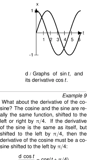
Figure d shows the graphs of the func-tion and its derivative. Note how the two graphs correspond. At t = 0, the slope of sint is at its largest, and is positive; this is where the deriva-tive, cost, attains its maximum posi-tive value of 1. Att = π/2, sint has reached a maximum, and has a slope of zero; cost is zero here. Att = π, in the middle of the graph, sinthas its maximum negative slope, and costis at its most negative extreme of−1. Physically, sint could represent the position of a pendulum as it moved back and forth from left to right, and cost would then be the pendulum’s velocity.
d/Graphs of sint, and its derivative cost.
Example 9 What about the derivative of the co-sine? The cosine and the sine are re-ally the same function, shifted to the left or right by π/4. If the derivative of the sine is the same as itself, but shifted to the left by π/4, then the derivative of the cosine must be a co-sine shifted to the left byπ/4:
d cost
e/Bishop George Berkeley (1685-1753)
2.2
Safe use of
infinitesimals
The idea of infinitesimally small numbers has always irked purists. One prominent critic of the cal-culus was Newton’s contemporary George Berkeley, the Bishop of Cloyne. Although some of his complaints are clearly wrong (he denied the possibility of the sec-ond derivative), there was clearly something to his criticism of the infinitesimals. He wrote sarcas-tically, “They are neither finite quantities, nor quantities infinitely small, nor yet nothing. May we not call them ghosts of departed quan-tities?”
Infinitesimals seemed scary, be-cause if you mishandled them, you could prove absurd things. For example, let du be an infinitesi-mal. Then 2du is also infinites-imal. Therefore both 1/du and 1/(2du) equal infinity, so 1/du = 1/(2du). Multiplying by du on both sides, we have a proof that 1 = 1/2.
In the eighteenth century, the use of infinitesimals became like adul-tery: commonly practiced, but shameful to admit to in polite cir-cles. Those who used them learned certain rules of thumb for handling them correctly. For instance, they would identify the flaw in my proof of 1 = 1/2 as my assumption that there was only one size of infinity, when actually 1/dushould be in-terpreted as an infinity twice as big as 1/(2du). The use of the sym-bol ∞ played into this trap, be-cause the use of a single symbol for infinity implied that infinities only came in one size. However, the practitioners of infinitesimals had trouble articulating a clear set of principles for their proper use, and couldn’t prove that a self-consistent system could be built around them.
By the twentieth century, when I learned calculus, a clear con-sensus had existed that infinite and infinitesimal numbers weren’t numbers at all. A notation like dx/dt, my calculus teacher told me, wasn’t really one number di-vided by another, it was merely a symbol for the limit
lim ∆t→0
∆x
∆t ,
where ∆x and ∆t represented fi-nite changes. That satisfied me un-til we got to a certain topic (im-plicit differentiation) in which we were encouraged to break the dx
2.2. SAFE USE OF INFINITESIMALS 27
buttonholed my teacher after class and asked why he was now doing what he’d told me you couldn’t re-ally do, and his response was that dxand dt weren’t really numbers, but most of the time you could get away with treating them as if they were, and you would get the right answer in the end. Most of the time!? That bothered me. How was I supposed to know when it
wasn’t “most of the time?”
f/Abraham Robinson (1918-1974)
But unknown to me and my teacher, mathematician Abraham Robinson had already shown in the 1960’s that it was possible to con-struct a self-consistent number sys-tem that included infinite and in-finitesimal numbers. He called it the hyperreal number system, and it included the real numbers as a subset.2
2The reader who wants to
learn more about the hyperreal system might want to start by reading K. Stroyan’s articles at
Moreover, the rules for what you can and can’t do with the hy-perreals turn out to be extremely simple. Take any true statement about the real numbers. Suppose it’s possible to translate it into a statement about the hyperreals in the most obvious way, simply by replacing the word “real” with the word “hyperreal.” Then the trans-lated statement is also true. This is known as thetransfer principle. Let’s look back at my bogus proof of 1 = 1/2 in light of this sim-ple princisim-ple. The final step of the proof, for example, is perfectly valid: multiplying both sides of the equation by the same thing. The following statement about the real numbers is true:
For any real numbersa,b, and
c, ifa=b, thenac=bc. This can be translated in an obvi-ous way into a statement about the hyperreals:
For any hyperreal numbersa,
b, andc, ifa=b, thenac=bc. However, what about the state-ment that both 1/duand 1/(2du)
http://www.math.uiowa.edu/~stroyan/ InfsmlCalculus/InfsmlCalc.htm. For more depth, one could next read the relevant parts of Keisler’s Elemen-tary Calculus: An Approach Using Infinitesimals, an out-of-print calculus text that uses infinitesimals, available for free from the author’s web site at
equal infinity, so they’re equal to each other? This isn’t the trans-lation of a statement that’s true about the reals, so there’s no rea-son to believe it’s true — and in fact it’s false.
What the transfer principle tells us is that the real numbers as we nor-mally think of them are not unique in obeying the ordinary rules of al-gebra. There are completely dif-ferent systems of numbers, such as the hyperreals, that also obey them.
How, then, are the hyperreals even different from the reals, if every-thing that’s true of one is true of the other? But recall that the transfer principle doesn’t guaran-tee that every statement about the reals is also true of the hyperre-als. It only works if the statement about the reals can be translated into a statement about the hyper-reals in the most simple, straight-forward way imaginable, simply by replacing the word “real” with the word “hyperreal.” Here’s an ex-ample of a true statement about the reals that can’t be translated in this way:
For any real number a, there is an integern that is greater thana.
This one can’t be translated so simplemindedly, because it refers to a subset of the reals called the integers. It might be possi-ble to translate it somehow, but it would require some insight into
the correct way to translate that word “integer.” The transfer prin-ciple doesn’t apply to this state-ment, which indeed is false for the hyperreals, because the hyperre-als contain infinite numbers that are greater than all the integers. In fact, the contradiction of this statement can be taken as a def-inition of what makes the hyper-reals special, and different from the reals: we assume that there is at least one hyperreal number,H, which is greater than all the inte-gers.
As an analogy from everyday life, consider the following statements about the student body of the high school I attended:
1. Every student at my high school had two eyes and a face. 2. Every student at my high school who was on the football team was a jerk.
2.2. SAFE USE OF INFINITESIMALS 29
and it’s not obvious what the cor-responding subset of Californians would be. Would it include ev-erybody who played high school, college, or pro football? Maybe it shouldn’t include the pros, be-cause they belong to an organiza-tion covering a region bigger than California. Statement 2 is the kind of statement that the transfer prin-ciple doesn’t apply to.3
Example 10 As a nontrivial example of how to ap-ply the transfer principle, let’s consider how to handle expressions like the one that occurred when we wanted to differentiatet2using infinitesimals:
d`
t2´
dt = 2t+ dt .
I argued earlier than 2t+ dtis so close to 2tthat for all practical purposes, the answer is really 2t. But is it really valid in general to say that 2t+ dt is the same hyperreal number as 2t? No. We can apply the transfer principle to the following statement about the re-als:
For any real numbers a and b, withb6= 0,a+b6=a.
Since dtisn’t zero, 2t+ dt6= 2t.
3For a slightly more precise and
for-mal statement of the transfer principle, the idea being expressed here is that the phrases “for any” and “there exists” can only be used in phrases like “for any real numberx” and “there exists a real num-ber y such that. . . ” The transfer prin-ciple does not apply to statements like “there exists an integerxsuch that. . . ” or even “there exists a subset of the real numbers such that. . . ”
More generally, example 10 leads us to visualize every number as be-ing surrounded by a “halo” of num-bers that don’t equal it, but dif-fer from it by only an infinitesi-mal amount. Just as a magnify-ing glass would allow you to see the fleas on a dog, you would need an infinitely strong microscope to see this halo. This is similar to the idea that every integer is sur-rounded by a bunch of fractions that would round off to that inte-ger. We can, however, define the
standard part of a finite hyperreal number, which means the unique real number that differs from it infinitesimally. For instance, the standard part of 2t+ dt, notated st(2t+ dt), equals 2t. The deriva-tive of a function should actually be defined as the standard part of dx/dt, but we often write dx/dt
to mean the derivative, and don’t worry about the distinction.
about the hyperreals was that they contain at least one infinite num-ber, H, which is bigger than all the integers. If this is true, then 1/H must be less than 1/2, less than 1/100, less then 1/1, 000, 000 — less than 1/nfor any integern. Therefore the hyperreals are guar-anteed to include infinitesimals as well, and so we have at least three levels to the hierarchy: infinities comparable to H, finite numbers, and infinitesimals comparable to 1/H. If you can swallow that, then it’s not too much of a leap to add more rungs to the ladder, like extra-small infinitesimals that are comparable to 1/H2. If this seems a little crazy, it may comfort you to think of statements about the hyperreals as descriptions of limit-ing processes involvlimit-ing real num-bers. For instance, in the sequence of numbers 1.12 = 1.21, 1.012 = 1.0201, 1.0012= 1.002001, . . . , it’s clear that the number represented by the digit 1 in the final decimal place is getting smaller faster than the contribution due to the digit 2 in the middle.
One subtle issue here, which I al-luded to in the differentiation of the sine function on page 25, is whether the transfer principle is sufficient to let us define all the functions that appear as familiar keys on a calculator: x2,√x, sinx, cosx, ex, and so on. After all, these functions were originally de-fined as rules that would take a real number as an input and give a
real number as an output. It’s not trivially obvious that their defini-tions can naturally be extended to take a hyperreal number as an in-put and give back a hyperreal as an output. Essentially the answer is that we can apply the transfer principle to them just as we would to statements about simple arith-metic, but I’ve discussed this a lit-tle more on page 105.
2.3
The product rule
When I first learned calculus, it seemed to me that if the deriva-tive of 3t was 3, and the deriva-tive of 7t was 7, then the deriva-tive of t multiplied by t ought to be just plain old t, not 2t. The reason there’s a factor of 2 in the correct answer is that t2 has two reasons to grow ast gets bigger: it grows because the first factor of t
is increasing, but also because the second one is. In general, it’s pos-sible to find the derivative of the product of two functions any time we know the derivatives of the in-dividual functions.
The product rule
Ifxandy are both functions oft, then the derivative of their product is
2.3. THE PRODUCT RULE 31
the productxyby an amount (x+ dx)(y+ dy)−xy
=ydx+xdy+ dxdy ,
and dividing by dt makes this into dx
dt ·y+x·
dy
dt +
dxdy
dt ,
whose standard part is the result to be proved.
Example 11
. Find the derivative of the function tsint.
.
d(tsint) dt =t·
d(sint) dt +
dt dt ·sint =tcost+ sint
Figure g gives the geometrical in-terpretation of the product rule. Imagine that the king, in his cas-tle at the southwest corner of his rectangular kingdom, sends out a line of infantry to expand his terri-tory to the north, and a line of cav-alry to take over more land to the east. In a time interval dt, the cav-alry, which moves faster, covers a distance dxgreater than that cov-ered by the infantry, dy. However, the strip of territory conquered by the cavalry, ydx, isn’t as great as it could have been, because in our exampleyisn’t as big asx.
g/A geometrical interpretation of the product rule.
A helpful feature of the Leibniz notation is that one can easily use it to check whether the units of an answer make sense. If we measure distances in meters and time in seconds, thenxyhas units of square meters (area), and so does the change in the area, d(xy). Dividing by dt gives the number of square meters per second be-ing conquered. On the right-hand side of the product rule, dx/dt
has units of meters per second (velocity), and multiplying it by
Because this unit-checking feature is so helpful, there is a special way of writing a second derivative in the Leibniz notation. What New-ton called ¨x, Leibniz wrote as
d2x
dt2 .
Although the different placement of the 2’s on top and bottom seems strange and inconsistent to many beginners, it actually works out nicely. If x is a distance, mea-sured in meters, and t is a time, in units of seconds, then the sec-ond derivative is supposed to have units of acceleration, in units of meters per second per second, also written (m/s)/s, or m/s2. (The acceleration of falling objects on Earth is 9.8 m/s2 in these units.) The Leibniz notation is meant to suggest exactly this: the top of the fraction looks like it has units of meters, because we’re not squaring
x, while the bottom of the fraction looks like it has units of seconds, because it looks like we’re squar-ing dt. Therefore the units come out right. It’s important to realize, however, that the symbol d isn’t a number (not a real one, and not a hyperreal one, either), so we can’t really square it; the notation is not to be taken as a literal statement about infinitesimals.
Example 12 A tricky use of the product rule is to find the derivative of√t. Since√tcan be written as t1/2
, we might suspect that the rule d(tk)
/dt = k tk−1 would
work, giving a derivative 12t−1/2 = 1/(2√t). However, the methods used to prove that rule in chapter 1 only work ifkis an integer, so the best we could do would be to confirm our con-jecture approximately by graphing. Using the product rule, we can write f(t) = d√t/dtfor our unknown deriva-tive, and back into the result using the product rule:
dt dt =
d(√t√t) dt
=f(t)√t+√tf(t) = 2f(t)√t
But dt/dt = 1, so f(t) = 1/(2√t) as claimed.
2.4. THE CHAIN RULE 33
h/Three clowns on seesaws demonstrate the chain rule.
2.4
The chain rule
Figure h shows three clowns on see-saws. If the leftmost clown moves down by a distance dx, the middle one will come up by dy, but this will also cause the one on the right to move down by dz. If we want to predict how much the rightmost clown will move in response to a certain amount of motion by the leftmost one, we have
dz
dx=
dz
dy ·
dy
dx .
This relation, called the chain rule, allows us to calculate a derivative of a function defined by one func-tion inside another. The proof, given on page 106, is essentially just the application of the trans-fer principle. (As is often the case, the proof using the hyperreals is much simpler than the one using real numbers and limits.)
Example 13
. Find the derivative of the function z(x) = sin(x2).
. Let y(x) = x2, so that z(x) =
sin(y(x)). Then
dz dx =
dz dy ·
dy dx = cos(y)·2x = 2xcos(x2)
2.5
Exponentials and
logarithms
The exponential
An important application of the chain rule comes up when we want to differentiate the omnipresent functionex, wheree= 2.71828. . . is the base of natural logarithms. We have just be a constant. Therefore we know that the derivative of ex is simplyex, multiplied by some un-known constant,
dex dx =c e
x .
A rough check by graphing at, say
x= 0, shows that the slope is close to 1, so c is close to 1. But how do we know it’s exactly one? The proof is given on page 106.
Example 14
.The concentration of a foreign sub-stance in the bloodstream generally falls off exponentially with time asc= coe−t/a, wherecois the initial
concen-tration, andais a constant. For caf-feine in adults, a is typically about 7 hours. An example is shown in figure i. Differentiate the concentration with respect to time, and interpret the re-sult. Check that the units of the result make sense.
.Using the chain rule, dc
This can be interpreted as the rate at which caffeine is being removed from the blood and put into the per-son’s urine. It’s negative because the concentration is decreasing. Accord-ing to the original expression for x, a substance with a large a will take a long time to reduce its concentra-tion, sincet/a won’t be very big un-less we have larget on top to com-pensate for the largeaon the bottom. In other words, larger values ofa rep-resent substances that the body has a harder time getting rid of efficiently. The derivative has a on the bottom, and the interpretation of this is that for a drug that is hard to eliminate, the rate at which it is removed from the blood is low.
2.5. EXPONENTIALS AND LOGARITHMS 35
the units are concentration divided by time, because the result represents the rate at which the concentration is changing.
i/Example 14. A typ-ical graph of the con-centration of caffeine in the blood, in units of mil-ligrams per liter, as a function of time, in hours.
Example 15
. Find the derivative of the function y= 10x.
.In general, one of the tricks to do-ing calculus is to rewrite functions in forms that you know how to handle. This one can be rewritten as a base-10 logarithm:
Applying the chain rule, we have the derivative of the exponential, which is just the same exponential, multiplied by the derivative of the inside stuff:
dy dx =e
xln 10
·ln 10 .
In other words, the “c” referred to in the discussion of the derivative ofex becomesc = ln 10 in the case of the base-10 exponential.
The logarithm
The natural logarithm is the func-tion that undoes the exponential. In a situation like this, we have
dy
dx=
1
dx/dy ,
where on the left we’re thinking of
y as a function of x, and on the right we considerxto be a function ofy. Applying this to the natural logarithm,
later. The proof is example 16 be-low.) The integral of x−1 is not
x0/0, which wouldn’t make sense anyway because it involves divi-sion by zero.4 Likewise the deriva-tive of x0 = 1 is 0x−1, which is zero. Figure j shows the idea. The functionsxn form a kind of ladder, with differentiation taking us down one rung, and integration taking us up. However, there are two special cases where differentiation takes us off the ladder entirely.
Example 16
.Prove d(xn)/dx=nxn−1for any real value ofn.
.
y=xn =enlnx
4Speaking casually, one can say that
division by zero gives infinity. This is often a good way to think when try-ing to connect mathematics to reality. However, it doesn’t really work that way according to our rigorous treatment of the hyperreals. Consider this statement: “For a nonzero real number a, there is no real numberbsuch thata= 0b.” This means that we can’t divideaby 0 and get b. Applying the transfer principle to this statement, we see that the same is true for the hyperreals: division by zero is un-defined. However, we can divide a finite number by an infinitesimal, and get an infinite result, which is almost the same thing.
j/Differentiation and integration of functions of the form xn. Constants out in front of the functions are not shown, so keep in mind that, for ex-ample, the derivative ofx2isn’tx, it’s
2x.
By the chain rule,
dy dx =e
nlnx
·n x
=xn·n x =nxn−1 .
(Forn= 0, the result is zero.)
When I started the discussion of the derivative of the logarithm, I wrote y = lnx right off the bat. That meant I was implicitly as-sumingxwas positive. More gen-erally, the derivative of ln|x|equals 1/x, regardless of the sign (see problem 24 on page 49).
2.6
Quotients
2.6. QUOTIENTS 37
on knowledge of the derivatives of the parts. We know how to find the derivatives of sums, differences, and products, so the obvious next step is to look for a way of handling division. This is straightforward, since we know that the derivative of the function function 1/u=u−1
and by the chain rule, d(v/u)
This is so easy to rederive on de-mand that I suggest not memoriz-ing it.
By the way, notice how the no-tation becomes a little awkward when we want to write a derivative like d(v/u)/dx. When we’re differ-entiating a complicated function, it can be uncomfortable trying to cram the expression into the top of the d. . . /d. . . fraction. Therefore it would be more common to write such an expression like this:
d dx
v
u
This could be considered an abuse of notation, making d look like a number being divided by another number dx, when actually d is meaningless on its own. On the other hand, we can consider the symbol d/dxto represent the op-eration of differentiation with re-spect to x; such an interpretation
will seem more natural to those who have been inculcated with the taboo against considering infinites-imals as numbers in the first place. Using the new notation, the quo-tient rule becomes
d
The interpretation of the minus sign is that ifuincreases,v/u de-creases.
Example 17
. Differentiate y = x/(1 + 3x), and check that the result makes sense.
.We identifyvwithxanduwith 1 +x. The result is
d
then the 1 would have to represent 1 gallon, since you can’t add things that have different units.) The functionyis defined by an expression with units of gallons divided by gallons, soyis unit-less. Therefore the derivative dy/dx should have units of inverse gallons. Both terms in the expression for the derivative do have those units, so the units of the answer check out.
2.7
Differentiation on
a computer
In this chapter you’ve learned a set of rules for evaluating derivatives: derivatives of products, quotients, functions inside other functions, etc. Because these rules exist, it’s always possible to find a formula for a function’s derivative, given the formula for the original function. Not only that, but there is no real creativity required, so a computer can be programmed to do all the drudgery. For example, you can download a free, open-source program called Yacas from
yacas.sourceforge.net and install it on a Windows or Linux machine. There is even a version you can run in a web browser with-out installing any special software:
http://yacas.sourceforge.net/ yacasconsole.html .
A typical session with Yacas looks like this:
Upright type represents your in-put, and italicized type is the pro-gram’s output.
First I asked it to differentiatex2 with respect to x, and it told me the result was 2x. Then I did the derivative of ex2, which I also could have done fairly easily by hand. (If you’re trying this out on a computer as you real along, make sure to capitalize functions like Exp, Sin, and Cos.) Finally I tried an example where I didn’t know the answer off the top of my head, and that would have been a little tedious to calculate by hand. Unfortunately things are a little less rosy in the world of integrals. There are a few rules that can help you do integrals, e.g., that the inte-gral of a sum equals the sum of the integrals, but the rules don’t cover all the possible cases. Using Ya-cas to evaluate the integrals of the same functions, here’s what hap-pens.5
5If you’re trying these on your own
2.7. DIFFERENTIATION ON A COMPUTER 39
Integrate(x)
Sin(Cos(Sin(x)))
The first one works fine, and I can easily verify that the answer is correct, by taking the derivative of x3/3, which is x2. (The an-swer could have beenx3/3 + 7, or
x3/3+c, wherecwas any constant, but Yacas doesn’t bother to tell us that.) The second and third ones don’t work, however; Yacas just spits back the input at us without making any progress on it. And it may not be because Yacas isn’t smart enough to figure out these integrals. The function ex2 can’t be integrated at all in terms of a formula containing ordinary oper-ations and functions such as ad-dition, multiplication, exponentia-tion, trig functions, exponentials, and so on.
That’s not to say that a program like this is useless. For example, here’s an integral that I wouldn’t have known how to do, but that Yacas handles easily:
Example 20
Integrate(x) Sin(Ln(x))
(x*Sin(Ln(x)))/2 -(x*Cos(Ln(x)))/2
This one is easy to check by dif-ferentiating, but I could have been marooned on a desert island for a decade before I could have figured it out in the first place. There are various rules, then, for integration, but they don’t cover all possible cases as the rules for differentiation do, and sometimes it isn’t obvious which rule to apply. Yacas’s ability
to integrate sin lnxshows that it had a rule in its bag of tricks that I don’t know, or didn’t remember, or didn’t realize applied to this in-tegral.
Back in the 17th century, when Newton and Leibniz invented cal-culus, there were no computers, so it was a big deal to be able to find a simple formula for your result. Nowadays, however, it may not be such a big deal. Suppose I want to find the derivative of sin cos sinx, evaluated atx= 1. I can do some-thing like this on a calculator:
Example 21
Example 22
(I’ve omitted all of Yacas’s output except for the final result.) Line 1 defines the function we want to differentiate. Lines 2 and 3 give values to the variables x and dx. Line 4 computes the derivative; the
N( ) surrounding the whole thing is our way of telling Yacas that we want an approximate numerical re-sult, rather than an exact symbolic one.
An interesting thing to try now is to make dx smaller and smaller, and see if we get better and bet-ter accuracy in our approximation to the derivative.
Example 23
5 g(x,dx):=
N( (f(x+dx)-f(x))/dx )
6 g(x,.1)
Line 5 defines the derivative func-tion. It needs to know both x and dx. Line 6 computes the derivative using dx= 0.1, which we expect to be a lousy approximation, since dx
is really supposed to be infinitesi-mal, and 0.1 isn’t even that small. Line 7 does it with the same value
of dxwe used earlier. The two re-sults agree exactly in the first dec-imal place, and approximately in the second, so we can be pretty sure that the derivative is −0.32 to two figures of precision. Line 8 ups the ante, and produces a re-sult that looks accurate to at least 3 decimal places. Line 9 attempts to produce fantastic precision by using an extremely small value of dx. Oops — the result isn’t bet-ter, it’s worse! What’s happened here is that Yacas computedf(x) and f(x+ dx), but they were the same to within the precision it was using, sof(x+ dx)−f(x) rounded off to zero.6
Example 23 demonstrates the con-cept of how a derivative can be de-fined in terms of a limit:
dy
dx = lim∆x→0 ∆y
∆x
The idea of the limit is that we can theoretically make ∆y/∆x ap-proach as close as we like to dy/dx, provided we make ∆x sufficiently small. In reality, of course, we eventually run into the limits of our ability to do the computation, as in the bogus result generated on line 9 of the example.
6Yacas can do arithmetic to any
2.9. LIMITS 41
2.8
Continuity
Intuitively, a continuous function is one whose graph has no sudden jumps in it; the graph is all a single connected piece. Formally, f(x) is defined to be continuous if for any realxand any infinitesimal dx,
f(x+ dx)−f(x) is infinitesimal. Example 24 Let the functionf be defined byf(x) = 0 forx ≤ 0, andf(x) = 1 forx > 0. Thenf(x) is discontinuous, since for dx>0,f(0 + dx)−f(0) = 1, which isn’t infinitesimal.
If a function is discontinuous at a given point, then it is not differen-tiable at that point. On the other hand, a function likey=|x|shows that a function can be continuous without being differentiable. Another way of thinking about continuous functions is given by the intermediate value theorem. Intuitively, it says that if you are moving continuously along a road, and you get from point A to point B, then you must also visit every other point along the road; only by teleporting (by moving discontin-uously) could you avoid doing so. More formally, the theorem states that if y is a continuous function on the interval from a to b, and if y takes on values y1 and y2 at certain points within this interval, then for anyy3betweeny1andy2, there is some xin the interval for whichy(x) =y3.7
7For a proof of the intermediate value
2.9
Limits
Historically, the calculus of in-finitesimals as created by New-ton and Leibniz was reinterpreted in the nineteenth century by Cauchy, Bolzano, and Weierstrass in terms of limits. All mathemati-cians learned both languages, and switched back and forth between them effortlessly, like the lady I overheard in a Southern California supermarket telling her mother, “Let’s get that one,con los nuts.” Those who had been trained in in-finitesimals might hear a statement using the language of limits, but translate it mentally into infinites-imals; to them, every statement about limits was really a state-ment about infinitesimals. To their younger colleagues, trained using limits, every statement about in-finitesimals was really to be under-stood as shorthand for a limiting process. When Robinson laid the rigorous foundations for the hyper-real number system in the 1960’s, a common objection was that it was really nothing new, because ev-ery statement about infinitesimals was really just a different way of expressing a corresponding state-ment about limits; of course the same could have been said about Weierstrass’s work of the preced-ing century! In reality, all prac-theorem starting from our definition of continuity, see Keisler’s Elemen-tary Calculus: An Approach Using Infinitesimals, p. 162, available online at
titioners of calculus had realized all along that different approaches worked better for different prob-lems; problem 11 on page 64 is an example of a result that is much easier to prove with infinitesimals than with limits.
The Weierstrass definition of a limit is this:
Definition of the limit
We say that ` is the limit of the function f(x) as x approaches a, written
lim
x→af(x) =` ,
if the following is true: for any real number, there exists another real numberδsuch that for allxin the intervala−δ≤x≤a+δ, the value off lies within the range from`−
to`+.
Intuitively, the idea is that if I want you to makef(x) close to`, I just have to tell you how close, and you can tell me that it will be that close as long asxis within a certain dis-tance ofa.
In terms of infinitesimals, we have:
Definition of the limit
We say that ` is the limit of the function f(x) as x approaches a, written
lim
x→af(x) =` ,
if the following is true: for any in-finitesimal number dx, f(x+ dx)
is finite, and the standard part of
f(x+ dx) equals`.
Sometimes a limit can be evaluated simply by plugging in numbers:
Example 25
L’H ˆopital’s rule
Consider the limit lim x→0
sinx
x .
2.9. LIMITS 43
Since plugging in zero didn’t work, let’s try estimating the limit by plugging in a number for xthat’s small, but not zero. On a calcula-tor,
sin 0.00001
0.00001 = 0.999999999983333 . It looks like the limit is 1. We can confirm our conjecture to higher precision using Yacas’s ability to do high-precision arithmetic:
N(Sin(10^-20)/10^-20,50)
0.99999999999999999 9999999999999999999 99998333333333
It’s looking pretty one-ish. This is the idea of the Weierstrass defini-tion of a limit: it seems like we can get an answer as close to 1 as we like, if we’re willing to make xas close to 0 as necessary.
But we still haven’t proved that the limit is exactly 1. Let’s try using the definition of the limit in terms of infinitesimals.
lim
This is a special case of a the fol-lowing rule for calculating limits involving 0/0:
L’Hˆopital’s rule
If u and v are functions with
u(a) = 0 and v(a) = 0, and the means that in Old French it used to be spelled and pronounced “L’Hospital,” but the “s” became silent, so they stopped writing it. So yes, it is the same word as
“hos-.Taking the derivatives of the top and bottom, we findex/1, which equals 1
when evaluated atx= 0.
In the following example, we have to use L’Hˆopital’s rule twice before we get an answer.
Example 27
.Applying L’H ˆopital’s rule gives −sinx
which still produces 0/0 when we plug
Another perspective on indeterminate forms
An expression like 0/0, called an indeterminate form, can be thought of in a different way in terms of infinitesimals. Suppose I tell you I have two infinitesimal numbers d and e in my pocket, and I ask you whether d/e is fi-nite, infifi-nite, or infinitesimal. You can’t tell, because d and e might not be infinitesimals of the same order of magnitude. For instance, if e = 37d, then d/e = 1/37 is fi-nite; but if e=d2, thend/e is in-finite; and if d = e2, then d/e is infinitesimal. Acting this out with numbers that are small but not in-finitesimal,
.000001 = 1000 .000001
.001 = .001 . On the other hand, suppose I tell you I have an infinitesimal num-ber d and a finite number x, and I ask you to speculate about d/x. You know for sure that it’s going to be infinitesimal. Likewise, you can be sure thatx/dis infinite. These aren’t indeterminate forms.
We can do something similar with infinite numbers. If H and K are both infinite, thenH−K is inde-terminate. It could be infinite, for example, ifH was positive infinite andK=H/2. On the other hand, it could be finite if H = K+ 1. Acting this out with big but finite numbers,
1000−500 = 500 1001−1000 = 1 .
Example 28
. If H is a positive infinite number, is√H+ 1−√H−1 finite, infinite, in-finitesimal, or indeterminate?
.Trying it with a finite, big number, we have
√
1000001−√999999
= 1.00000000020373×10⁻³ , which is clearly a wannabe infinitesi-mal. More rigorously, we can rewrite the expression as √H(p1 + 1/H −
p
1−1/H). Since the derivative of the square root function√xevaluated atx = 1 is 1/2, we can approximate
which is clearly infinitesimal.
2.9. LIMITS 45
Example 29
.Evaluate the limit
lim
x→∞
2x+ 7 x+ 8686 .