841 Pro Spatial with SQL Server 2012

(1)

(2)

For your convenience Apress has placed some of the front

matter material after the index. Please use the Bookmarks

(3)

Contents at a Glance

Contents...vii

Foreword ... xxi

About the Author ... xxii

About the Technical Reviewer ... xxiii

Acknowledgments ... xxiv

Introduction ... xxv

■

Chapter 1: Spatial Reference Systems...1

■

Chapter 2: Spatial Features ...21

■

Chapter 3: Spatial Datatypes ...51

■

Chapter 4: Creating Spatial Data...77

■

Chapter 5: Importing Spatial Data ...101

■

Chapter 6: Geocoding...139

■

Chapter 7: Precision, Validity, and Errors...163

■

Chapter 8: Transformation and Reprojection...187

■

Chapter 9: Examining Spatial Properties ...211

■

Chapter 10: Modification and Simplification ...253

■

Chapter 11: Aggregation and Combination ...273

■

Chapter 12: Testing Spatial Relationships ...293

(4)

■

Chapter 14: Route Finding ...353

■

Chapter 15: Triangulation and Tesselation ...387

■

Chapter 16: Visualization and User Interface ...419

■

Chapter 17: Reporting Services ...445

■

Chapter 18: Indexing...471

■

Appendix ...499

(5)

C H A P T E R 1

■ ■ ■

Spatial Reference Systems

Spatial data analysis is a complex subject area, taking elements from a range of academic disciplines, including geophysics, mathematics, astronomy, and cartography. Although you do not need to understand these subjects in great depth to take advantage of the spatial features of SQL Server 2012, it is important to have a basic understanding of the theory involved so that you use spatial data appropriately and effectively in your applications.

This chapter describes spatial reference systems—ways of describing positions in space—and shows how these systems can be used to define features on the earth's surface. The theoretical concepts discussed in this chapter are fundamental to the creation of consistent, accurate spatial data, and are used throughout the practical applications discussed in later chapters of this book.

What Is a Spatial Reference System?

The purpose of a spatial reference system (sometimes called a coordinate reference system) is to identify and unambiguously describe any point in space. You are probably familiar with the terms

latitude and longitude, and have seen them used to describe positions on the earth. If this is the case, you may be thinking that these represent a spatial reference system, and that a pair of latitude and longitude coordinates uniquely identifies every point on the earth's surface, but, unfortunately, it's not quite that simple.

What many people don't realize is that any particular point on the ground does not have a unique latitude or longitude associated with it. There are, in fact, many systems of latitude and longitude, and the coordinates of a given point on the earth will differ depending on which system was used.

Furthermore, latitude and longitude coordinates are not the only way to define locations: many spatial reference systems describe the position of an object without using latitude and longitude at all. For example, consider the following three sets of coordinates:

• 51.179024688899524, –1.82747483253479 • SU 1215642213

• 581957, 5670386

These coordinates look very different, yet they all describe exactly the same point on the earth's surface, located in Stonehenge, in Wiltshire, United Kingdom. The coordinates differ because they all relate to different spatial reference systems: the first set is latitude and longitude coordinates from the WGS84 reference system, the second is a grid reference from the National Grid of Great Britain, and the third is a set of easting/northing coordinates from UTM Zone 30U.

(6)

CHAPTER 1 ■ SPATIAL REFERENCE SYSTEMS

Many different spatial reference systems exist, and each has different benefits and drawbacks: some offer high accuracy but only over a relatively small geographic area; others offer reasonable accuracy across the whole globe. Some spatial reference systems are designed for particular purposes, such as for nautical navigation or for scientific use, whereas others are designed for general global use.

One key point to remember is that every set of coordinates is unique to a particular spatial reference system, and only makes sense in the context of that system.

Modeling the Earth

The earth is a very complex shape. On the surface, we can see by looking around us that there are irregular topographical features such as mountains and valleys. But even if we were to remove these features and consider the mean sea-level around the planet, the earth is still not a regular shape. In fact, it is so unique that geophysicists have a specific word solely used to describe the shape of the earth: the geoid.

The surface of the geoid is smooth, but it is distorted by variations in gravitational field strength caused by changes in the earth's composition. Figure 1-1 illustrates a depiction of the shape of the geoid.

Figure 1-1. The irregular shape of the earth.

In order to describe the location of an object on the earth’s surface with maximum accuracy, we would ideally define its position relative to the geoid itself. However, even though scientists have recently developed very accurate models of the geoid (to within a centimeter accuracy of the true shape of the earth), the calculations involved are very complicated. Instead, spatial reference systems normally define positions on the earth's surface based on a simple model that approximates the geoid. This approximation is called a reference ellipsoid.

(7)

Approximating the Geoid

Many early civilizations believed the world to be flat (and a handful of modern day organizations still do, e.g., the “Flat Earth Society,” http://www.theflatearthsociety.org). Our current understanding of the shape of the earth is largely based on the work of Ancient Greek philosophers and scientists, including Pythagoras and Aristotle, who scientifically proved that the world is, in fact, round. With this fact in mind, the simplest reference ellipsoid that can be used to approximate the shape of the geoid is a perfect sphere. Indeed, there are some spatial reference systems that do use a perfect sphere to model the geoid, such as the system on which many Web-mapping providers, including Google Maps and Bing Maps, are based.

Although a sphere would certainly be a simple model to use, it doesn't really match the shape of the earth that closely. A better model of the geoid, and the one most commonly used, is an oblate spheroid. A spheroid is the three-dimensional shape obtained when you rotate an ellipse about its shorter axis. In other words, it's a sphere that has been squashed in one of its dimensions. When used to model the earth, spheroids are always oblate—they are wider than they are high—as if someone sat on a beach ball. This is a fairly good approximation of the shape of the geoid, which bulges around the equator.

The most important property of a spheroid is that, unlike the geoid, a spheroid is a regular shape that can be exactly mathematically described by two parameters: the length of the semi-major axis (which represents the radius of the earth at the equator), and the length of the semi-minor axis (the radius of the earth at the poles). The properties of a spheroid are illustrated in Figure 1-2.

Figure 1-2. Properties of a spheroid.

(8)

The flattening ratio of an ellipsoid, f, is used to describe how much the ellipsoid has been “squashed,” and is calculated as

f = (a – b ) / a

where a = length of the semi-major axis; b = length of the semi-minor axis.

In most ellipsoidal models of the earth, the semi-minor axis is only marginally smaller than the semi-major axis, which means that the value of the flattening ratio is also small, typically around 0.003. As a result, it is sometimes more convenient to state the inverse flattening ratio of an ellipsoid instead. This is written as 1/f, and calculated as follows.

1 / f = a / (a – b)

The inverse-flattening ratio of an ellipsoid model typically has a value of approximately

300.Given the length of the semi-major axis a and any one other parameter, f, 1/f, or b, we have all the information necessary to describe a reference ellipsoid used to model the shape of the earth.

Regional Variations in Ellipsoids

There is not a single reference ellipsoid that best represents every part of the whole geoid. Some ellipsoids, such as the World Geodetic System 1984 (WGS84) ellipsoid, provide a reasonable approximation of the overall shape of the geoid. Other ellipsoids approximate the shape of the geoid very accurately over certain regions of the world, but are much less accurate in other areas. These local ellipsoids are normally only used in spatial reference systems designed for use in specific countries, such as the Airy 1830 ellipsoid commonly used in Britain, or the Everest ellipsoid used in India.

Figure 1-3 provides an (exaggerated) illustration of how different ellipsoid models vary in accuracy over different parts of the geoid. The dotted line represents an ellipsoid that provides the best accuracy over the region of interest, whereas the dash-dotted line represents the ellipsoid of best global accuracy.

(9)

It is important to realize that specifying a different reference ellipsoid to approximate the geoid will affect the accuracy with which a spatial reference system based on that ellipsoid can describe the position of features on the earth. When choosing a spatial reference system, we must therefore be careful to consider one that is based on an ellipsoid suitable for the data in question.

SQL Server 2012 recognizes spatial reference systems based on a number of different reference ellipsoids, which best approximate the geoid at different parts of the earth. Table 1-1 lists the

properties of some commonly used ellipsoids that can be used.

Table 1-1. Properties of Some Commonly Used Ellipsoids

Ellipsoid Name Semi-Major Axis (m) Semi-Minor Axis (m) Inverse Flattening Area of Use

Airy (1830) 6,377,563.396 6,356,256.909 299.3249646 Great Britain

Bessel (1841) 6,377,397.155 6,356,078.963 299.1528128 Czechoslovakia, Japan, South Korea

Clarke (1880) 6,378,249.145 6,356,514.87 293.465 Africa

NAD 27 6,378,206.4 6,356,583.8 294.9786982 North America

NAD 83 6,378,137 6,356,752.3 298.2570249 North America

WGS 84 6,378,137 6,356,752.314 298.2572236 Global

Realizing a Reference Ellipsoid Model with a Reference Frame

Having established the size and shape of an ellipsoid model, we need some way to position that model to make it line up with the correct points on the earth's surface. An ellipsoid is just an abstract

mathematical shape; in order to use it as the basis of a spatial reference system, we need to correlate coordinate positions on the ellipsoid with real-life locations on the earth. We do this by creating a frame of reference points.

Reference points are places (normally on the earth's surface) that are assigned known

coordinates relative to the ellipsoid being used. By establishing a set of points of known coordinates, we can use these to "realize" the reference ellipsoid in the correct position relative to the earth. Once the ellipsoid is set in place based on a set of known points, we can then obtain the coordinates of any other points on the earth, based on the ellipsoid model.

Reference points are sometimes assigned to places on the earth itself; The North American Datum of 1927 (NAD 27) uses the Clarke (1866) reference ellipsoid, primarily fixed in place at Meades Ranch in Kansas. Reference points may also be assigned to the positions of satellites orbiting the earth, which is how the WGS 84 datum used by GPS-positioning systems is realized.

When packaged together, the properties of the reference ellipsoid and the frame of reference points form a geodetic datum. The most common datum in global use is the World Geodetic System of 1984, commonly referred to as WGS 84. This is the datum used in handheld GPS systems, Google Earth, and many other applications.

A datum, consisting of a reference ellipsoid model combined with a frame of reference points, creates a usable model of the earth used as the basis for a spatial reference system.

(10)

There are many different sorts of coordinate systems, but when you use geospatial data in SQL Server 2012, you are most likely to use a spatial reference system based on either geographic or

projected coordinates.

Geographic Coordinate Systems

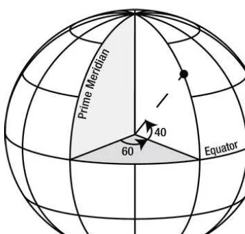
In a geographic coordinate system, any location on the surface of the earth can be defined using two coordinates: a latitude coordinate and a longitude coordinate.

The latitude coordinate of a point measures the angle between the plane of the equator and a line drawn perpendicular to the surface of the earth to that point.

The longitude coordinate measures the angle (in the equatorial plane) between a line drawn from the center of the earth to the point and a line drawn from the center of the earth to the prime meridian. The prime meridian

is an imaginary line drawn on the earth's surface between the North Pole and the South Pole (so technically it is an arc, rather than a line) that defines the axis from which angles of longitude are measured.

The definitions of the geographic coordinates of latitude and longitude are illustrated in Figure 1-4.

Figure 1-4. Describing positions using a geographic coordinate system.

(11)

Geographic Units of Measurement

Coordinates of latitude and longitude are both angles, and are usually measured in degrees (although they can be measured in radians or any other angular unit of measure). When measured in degrees, longitude values measured from the prime meridian range from –180° to +180°, and latitude values measured from the equator range from –90° (at the South pole) to +90° (at the North pole).

Longitudes to the east of the prime meridian are normally stated as positive values, or suffixed with the letter "E". Longitudes to the west of the prime meridian are expressed as negative values, or using the suffix "W". Likewise, latitudes north of the equator are expressed as positive values or using letter "N", whereas those south of the equator are negative or denoted with the letter "S".

NOTATION OF GEOGRAPHIC COORDINATES

There are several accepted methods of expressing coordinates of latitude and longitude.

When expressing geographic coordinate values of latitude and longitude for use in SQL Server 2012, you must always use decimal degree notation. The advantage of this format is that each coordinate can be expressed as a single floating-point number. To convert DMS coordinates into decimal degrees you can use the following rule.

Degrees + (Minutes / 60) + (Seconds / 3600) = Decimal Degrees

For example, the CIA World Factbook (https://www.cia.gov/library/publications/the-world-factbook/geos/uk.html ) gives the geographic coordinates for London as follows, 51 30 N, 0 10 W

When expressed in decimal degree notation, this is 51.5 (Latitude), –0.166667 (Longitude)

Defining the Origin of a Geographic Coordinate System

Latitude coordinates are always measured relative to the equator: the line that goes around the "middle" of the earth. But from where should longitude coordinates, which are measured around the earth, be measured?

1. The most commonly used method is the DMS (degree, minutes, seconds) system, also known as sexagesimal notation. In this system, each degree is divided into 60 minutes. Each minute is further subdivided into 60 seconds. A value of 51 degrees, 15 minutes, and 32 seconds is normally written as 51°15’32”.

2. An alternative system, commonly used by GPS receivers, displays whole degrees, followed by minutes and decimal fractions of minutes. This same coordinate value would therefore be written as 51:15.53333333.

(12)

A common misconception is to believe that there is a universal prime meridian based on some inherent fundamental property of the earth, but this is not the case. The prime meridian of any spatial reference system is arbitrarily chosen simply to provide a line of zero longitude from which all other coordinates of longitude can be calculated. The most commonly used prime meridian is the meridian passing through Greenwich, England, but there are many others. For example, the RT38 spatial reference system used in Sweden is based on a prime meridian that passes through Stockholm, some 18 degrees east of the Greenwich Prime Meridian. Prime meridians from which coordinates are measured in other systems include those that pass through Paris, Jakarta, Madrid, Bogota, and Rome.

If you were to define a different prime meridian, the value of the longitude coordinate of all the points in a given spatial reference system would change.

Projected Coordinate Systems

Describing the location of positions on the earth using coordinates of latitude and longitude is all very well in certain circumstances, but it's not without some problems. To start with, you can only apply angular coordinates onto a three-dimensional, round model of the earth. If you were planning a car journey you'd be unlikely to refer to a “travel globe” though, wouldn't you? Because an ellipsoidal model, by definition, represents the entire world, you can't magnify an area of interest without enlarging the entire globe. Clearly this would get unwieldy for any applications that required focusing in detail on a small area of the earth’s surface.

Fortunately, ancient geographers and mathematicians devised a solution for this problem, and the art of cartography, or map-making, was born. Using various techniques, a cartographer can project all, or part, of the surface of an ellipsoidal model onto a flat plane, creating a map. The features on that map can be scaled or adjusted as necessary to create maps suitable for different purposes.

Because a map is a flat, two-dimensional surface, we can then describe positions on the plane of that map using familiar two-dimensional Cartesian coordinates in the x- and y-axes. This is known as a projected coordinate system.

■Note In contrast to a geographic coordinate system, which defines positions on a three-dimensional, round model of the earth, a projected coordinate system describes the position of points on the earth’s surface as they lie on a flat, projected, two-dimensional plane.

Creating Map Projections

We see two-dimensional projections of geospatial data on an almost daily basis in street maps, road atlases, or on our computer screens. Given their familiarity, and the apparent simplicity of working on a flat surface rather than a curved one, you would be forgiven for thinking that defining spatial data using a projected coordinate system was somehow simpler than using a geographic coordinate system. The difficulty associated with a projected coordinate system is that, of course, the world isn’t a flat, two-dimensional plane. In order to be able to represent it as one, we have to use a map projection.

Projection is the process of creating a two-dimensional representation of a three-dimensional model of the earth, as illustrated in Figure 1-5. Map projections can be constructed either by using purely geometric methods (such as the techniques used by ancient cartographers) or by using

(13)

without distorting the resulting image in some way. Distortions introduced as a result of the projection process may affect the area, shape, distance, or direction represented by different elements of the map.

Figure 1-5. Projecting a 3D model of the earth to create a flat map.

By altering the projection method, cartographers can reduce the effect of these distortions for certain features, but in doing so the accuracy of other features must be compromised. Just as there is not a single "best" reference ellipsoid to model the three-dimensional shape of the earth, neither is there a single best map projection when trying to project that model onto a two-dimensional surface.

Over the course of time, many projections have been developed that alter the distortions introduced as a result of projection to create maps suitable for different purposes. For instance, when designing a map to be used by sailors navigating through the Arctic regions, a projection may be used that maximizes the accuracy of the direction and distance of objects at the poles of the earth, but sacrifices accuracy of the shape of countries along the equator.

The full details of how to construct a map projection are outside the scope of this book. However, the following sections introduce some common map projections and examine their key features.

Hammer–Aitoff Projection

(14)

Figure 1-6. The Hammer–Aitoff map projection.

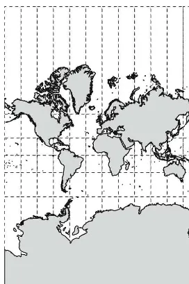
Mercator Projection

The Mercator map projection is an example of a conformal map projection. A conformal map projection is any projection that preserves the local shape of objects on the resulting map.

The Mercator projection was first developed in 1569 by the Flemish cartographer Gerardus Mercator, and has been widely used ever since. It is used particularly in nautical navigation because, when using any map produced using the Mercator projection, the route taken by a ship following a constant bearing will be depicted as a straight line on the map.

The Mercator projection accurately portrays all points that lie exactly on the equator. However, as you move farther away from the equator, the distortion of features, particularly the representation of their area, becomes increasingly severe. One common criticism of the Mercator projection is that, due to the geographical distribution of countries in the world, many developed countries are depicted with far greater area than equivalent-sized developing countries. For instance, examine Figure 1-7 to see how the relative sizes of North America (actual area 19 million sq km) and Africa (actual area 30 million sq km) are depicted as approximately the same size.

(15)

Figure 1-7. The Mercator map projection.

Equirectangular Projection

The equirectangular projection is one of the first map projections ever to be invented, being credited to Marinus of Tyre in about 100 AD. It is also one of the simplest map projections, in which the map displays equally spaced degrees of longitude on the x-axis, and equally spaced degrees of latitude on the y-axis.

(16)

as portraying NASA satellite imagery of the world (http://visibleearth.nasa.gov/). Figure 1-8 illustrates a map of the world created using the equirectangular projection method.

Figure 1-8. The equirectangular map projection.

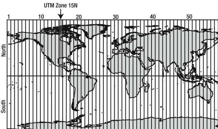
Universal Transverse Mercator Projection

The Universal Transverse Mercator (UTM) projection is not a single projection, but rather a grid composed of many projections laid side by side. The UTM grid is created by dividing the globe into 60 slices, called “zones,” with each zone being 6° wide and extending nearly the entire distance between the North Pole and South Pole (the grid does not extend fully to the polar regions, but ranges from a latitude of 80°S to 84°N). Each numbered zone is further subdivided by the equator into north and south zones. Any UTM zone may be referenced using a number from 1 to 60, together with a suffix of N or S to denote whether it is north or south of the equator. Figure 1-9 illustrates the grid of UTM zones overlaid on a map of the world, highlighting UTM Zone 15N.

(17)

Figure 1-9. UTM zones of the world.

The UTM projection is universal insofar as it defines a system that can be applied consistently across the entire globe. However, because each zone within the UTM grid is based on its own unique projection, the UTM map projection can only be used to represent accurately those features lying within a single specified zone.

Projection Parameters

In addition to the method of projection used, there are a number of additional parameters that affect the appearance of any projected map. These parameters are listed in Table 1-2.

Table 1-2. Map Projection Parameters

Parameter Description

Azimuth The angle at which the center line of the projection lies, relative to north

Central meridian The line of longitude used as the origin from which x coordinates are measured

False easting A value added to x coordinates so that stated coordinate values remain positive over the extent of the map

False northing A value added to y coordinates so that stated coordinate values remain positive over the extent of the map

(18)

Parameter Description

Latitude of origin The latitude used as the origin from which y coordinates are measured

Latitude of point The latitude of a specific point on which the map projection is based

Longitude of center The longitude of the point at the center of the map projection

Longitude of point The longitude of a specific point on which the map projection is based

Scale factor A scaling factor used to reduce the effect of distortion in a map projection

Standard parallel A line of latitude along which features on the map have no distortion

Projected Units of Measurement

Having done the hard work involved in creating a projection, the task of defining coordinates on that projection thankfully becomes much easier. If we consider all of the points on the earth’s surface to lie on the flat surface of a map then we can define positions on that map using familiar Cartesian coordinates of x and y, which represent the distance of a point from an origin along the x-axis and y -axis, respectively. In a projected coordinate system, these coordinate values are normally referred to as eastings (the x-coordinate) and northings (the y-coordinate). This concept is illustrated in Figure 1-10.

(19)

Eastings and northings coordinate values represent a linear distance east and north of a given origin. Although most projected coordinates are measured in meters, the appropriate units of

measurement for a spatial reference system will vary depending on the uses of that particular system. Some systems use imperial units of measurement or locally relevant units: the foot, Clarke's foot, the U.S. survey foot, or the Indian foot, for example (all of which are approximately equal to 30.5 cm, although subtly different!). The coordinates of a spatial reference system designed for high-accuracy local surveys may even specify millimeters as a unit of measurement.

Putting It All Together: Components of a Spatial Reference

System

We have examined several components that make up any spatial reference system—a system that allows us to define positions on the earth’s surface—that we can use to describe positions on the surface of the earth. Table 1-3 gives an overview of each component.

Table 1-3. Components of a Spatial Reference System

Component Function

Coordinate system Specifies a mathematical framework for determining the position of items relative to an origin. Coordinate systems used in SQL Server are generally either based on geographic or projected coordinate systems.

Datum States a model of the earth onto which we can apply the coordinate system. Consists of a reference ellipsoid (a three-dimensional mathematical shape that approximates the shape of the earth) and a reference frame (a set of points to position the reference ellipsoid relative to known locations on the earth).

Prime meridian Defines the axis from which coordinates of longitude are measured.

Projectiona _{Details the parameters required to create a two-dimensional image of the} earth’s surface (i.e., a map), so that positions can be defined using projected coordinates.

Unit of measurement Provides the appropriate unit in which coordinate values are expressed.

a_{Projection parameters are only defined for spatial reference systems based on projected coordinate systems.}

(20)

■ Note In order to be able to describe positions on the earth using a projected coordinate system, a spatial reference system must first specify a three-dimensional, geodetic model of the world (as would be used by a geographic coordinate system), and then additionally state the parameters detailing how the two-dimensional projected map image should be created from that model. For this reason, spatial reference systems based on projected coordinate systems must contain all the same elements as those based on geographic coordinate systems, together with the additional parameters required for the projection.

Spatial Reference Identifiers (SRIDs)

Every time we state the latitude and longitude, or x- and y-coordinates, that describe the position of a point on the earth, we must also state the associated spatial reference system from which those coordinates were obtained. Without the extra information contained in the spatial reference system, a coordinate tuple is just an abstract set of numbers in a mathematical system. The spatial reference system takes the abstract coordinates from a geographic or projected system and puts them in a context so that they can be used to identify a real position on the earth’s surface.

However, it would be quite cumbersome to have to write out the full details of the datum, the prime meridian, and the unit of measurement (and any applicable projection parameters) each time we wrote down a set of coordinates. Fortunately, various authorities allocate easily memorable, unique integer reference numbers that represent all of the necessary parameters of a spatial reference system. These reference numbers are called spatial reference identifiers (SRIDs).

One authority that allocates SRIDs is the European Petroleum Survey Group (EPSG), and its reference identification system is implemented in SQL Server 2012. Whenever you use any of the spatial functions in SQL Server that involve stating the coordinates of a position, you must also supply the relevant EPSG SRID of the system from which those coordinates were obtained.

Some examples of SRIDs assigned by the EPSG that can be used in SQL Server are:

• 4269 (North American Datum 1983) • 32601 (UTM Zone 1 North)

• 4326 (World Geodetic System 1984)

• 32136 (Tennessee State Plane Coordinate System)

A more comprehensive list of common spatial reference identifiers can be found in the appendix of this book.

(21)

Well-Known Text of a Spatial Reference System

SQL Server maintains a catalogue view, sys.spatial_reference_systems, in which it stores the details of all 392 supported geographic spatial reference systems. The information contained in this table is required to define the model of the earth on which geographic coordinate calculations take place. Note that no additional information is required to perform calculations of data defined using projected coordinates, because these take place on a simple 2D plane. Therefore SQL Server can support data defined using any projected coordinate system.

The parameters of each geographic spatial reference system in sys.spatial_reference_systems are stored in the well_known_text column using the Well-Known Text (WKT) format, which is an industry-standard format for expressing spatial information defined by the Open Geospatial Consortium (OGC).

■ Note SQL Server only supports geographic coordinate data defined relative to one of the spatial reference systems listed in sys.spatial_reference_systems. This table contains the additional information required to construct the model of the earth on which geographic coordinate calculations take place. However, because no additional information is required to perform calculations on a 2D plane, SQL Server supports projected coordinate data defined from any projected coordinate reference system, and the details of such systems are not listed in sys.spatial_reference_systems.

To illustrate how spatial references are represented in WKT format, let’s examine the properties of the EPSG:4326 spatial reference by executing the following query.

SELECT

well_known_text FROM

sys.spatial_reference_systems WHERE

authority_name = 'EPSG' AND

authorized_spatial_reference_id = 4326;

The following is the result (with line breaks and indents added to make the result easier to read).

GEOGCS[ "WGS 84", DATUM[

(22)

This result contains all the parameters required to define this spatial reference system, as follows.

Coordinate system: The first line of a WKT spatial reference is a keyword to tell us what sort of coordinate system is used. In this case, GEOGCS tells us that EPSG:4326 uses a geographic coordinate reference system. If a spatial reference system is based on projected coordinates then the WKT representation would instead begin with PROJCS. Immediately following this is the name assigned to the spatial reference system. In this case, the Well-Known Text is describing the "WGS 84" spatial reference system.

Datum: The values following the DATUM keyword provide the parameters of the datum. The first parameter gives us the name of the datum used. In this case, it is the "World Geodetic System 1984" datum. Then follow the parameters of the reference ellipsoid. This system uses the "WGS 84" ellipsoid, with a semimajor axis of 6,378,137 m and an inverse-flattening ratio of 298.257223563.

Prime meridian: The PRIMEM value tells us that this system defines Greenwich as the prime meridian, where longitude is defined to be 0.

Unit of measurement: The final parameter specifies that the unit in which coordinates are measured is the "Degree". The value of 0.0174532925199433 is a conversion factor required to convert from radians into the stated units (1 degree = π/180 radians).

Contrasting a Geographic and a Projected Spatial Reference

Let’s compare the result in the preceding section to the WKT representation of a spatial reference system based on a projected coordinate system. The following example shows the WKT representation of the UTM Zone 10N reference, a projected spatial reference system used in North America. The SRID for this system is EPSG:26910.

■Note Remember that, because this is a projected spatial reference system, you won't find these details in the sys.spatial_reference_systems table. Instead, you can look up the details of these systems using a site such as http://www.epsg-registry.org or http://www.spatialreference.org.

PROJCS[

"NAD_1983_UTM_Zone_10N", GEOGCS[

"GCS_North_American_1983", DATUM[

"D_North_American_1983", SPHEROID[

(23)

UNIT["Degree", 0.0174532925199433] ],

Notice that the Well-Known Text for this projected coordinate system contains a complete set of parameters for a geographic coordinate system, embedded within brackets following the GEOGCS keyword. The reason is that a projected system must first define the three-dimensional, geodetic model of the earth, and then specify several additional parameters that are required to project that model onto a plane.

■ Note The Well-Known Text format in which SQL Server stores the properties of spatial reference systems in the sys.spatial_reference_systems table is exactly the same format as used in the .PRJ file used to describe the spatial reference in which the data in an ESRI shapefile are stored.

Summary

After reading this chapter, you should understand how spatial reference systems can be used to describe positions in space:

• A spatial reference system consists of a coordinate system (which describes a position using either projected or geographic coordinates), a datum (which describes a model representing the shape of the earth), the prime meridian (which defines the origin from which units are measured), and the unit of measurement. When using projected coordinates, the spatial reference system also defines the properties of the projection used.

• A geographic coordinate system defines the position of objects using angular coordinates of latitude and longitude, which are measured from the equator and the prime meridian, respectively.

• A projected coordinate system defines the position of objects using Cartesian coordinates, which measure the x and y distance of a point from an origin. These are also referred to as easting and northing coordinates.

• Whenever you state a set of coordinates representing a point on the earth, it is essential that you also give details of the associated spatial reference system. The spatial reference system defines the additional information that allows us to apply the coordinate reference to identify a point on the earth.

(24)

• Details of all the geographic spatial reference systems supported by SQL Server 2012 are contained within a system catalogue view called

sys.spatial_reference_systems. SQL Server also supports data defined using any projected spatial reference system.

• The Well-Known Text format is a standard format used to express the properties of a spatial reference system.

If you are interested in reading further about the topics covered in this chapter, I recommend checking out the Microsoft white paper, "Introduction to Spatial Coordinate Systems: Flat Maps for a Round Planet," which can be found in the MSDN SQL Server developer center site, at

(25)

C H A P T E R 2

■ ■ ■

Spatial Features

In the last chapter, I stated that the purpose of geospatial data was to describe the shape and location of objects on the Earth. Although this objective may be simply stated, in practice it is not always so easy to achieve.

In many cases, although we have a rough understanding of the position and geographic extent of features on the Earth, they may be hard to define in exact terms. For example, at what point does the body of water known as the Gulf of Mexico become the Atlantic Ocean? Where exactly do we draw the line that defines the boundary of a city or forest? In some parts of the world, there is even ambiguity or contention as to where the border between two countries lies, and there are still significant areas of land and sea that are subjects of international dispute.

Even if we agree on the precise shape and location of a feature, it may be hard to describe the properties of that feature with sufficient detail; natural features, such as rivers and coastlines, have complex irregular shapes. Even man-made structures such as roads are rarely simple straight lines.

It would be very hard, if not impossible, to define the shape of these features exactly. Instead, spatial data represents these objects by storing simple geometrical shapes that approximate their actual shape and position. These shapes are called geometries.

The spatial functionality in SQL Server is based on the Open Geospatial Consortium’s “Simple Features for SQL Specification”, which you can view online at

http://www.opensgeospatial.org/standards/sfs. This standard defines a number of different types of geometries, each with different associated properties. In this chapter, each of the different types of geometry is examined and the situations in which it is most appropriate to use each type are described.

■Note In the context of spatial data, the word "geometry" can have two distinct meanings. To emphasize the difference, geometry (code formatting) is used to refer to the geometry datatype, whereas geometry (no formatting) is used to refer to simple shapes representing features on the Earth.

Geometry Hierarchy

There is a total of 14 standard types of geometries recognized by SQL Server (not counting the special cases of the FullGlobe or Empty geometries; more on those later). However, only ten of these geometry types are instantiable (that is to say, you can actually create instances of these geometries); the remaining four types are abstract classes from which other instantiable classes are derived.

(26)

CHAPTER 2 ■ SPATIAL FEATURES

Single geometries contain one discrete geometric element. The most basic single geometry is a Point. There are also three types of curve (LineString, CircularString, and CompoundCurve) and two types of surface (Polygon and CurvePolygon).

Geometry collections are compound elements, containing one or more of the individual geometries listed above. Geometry collections may be

homogeneous or heterogeneous. A homogeneous geometry collection contains several items of the same type of single geometry only (e.g., a MultiPoint is a geometry collection containing only Points). A heterogeneous geometry collection contains one or more of several different sorts of geometry, such as a collection containing a LineString and a Polygon.

■Note The Microsoft Books Online documentation refers to these two categories of geometries as “Simple types” and “Collection types”

(http://technet.microsoft.com/en-us/library/bb964711%28SQL.110%29.aspx). The use of the word “Simple” here has been deliberately avoided because this has a separate meaning (as used by the STIsSimple() method) that is discussed later.

Figure 2-1 illustrates the inheritance tree of geometry types, which demonstrates how the different types of geometry are related to each other. Every item of spatial data in SQL Server is an example of one of the ten instantiable classes shown with a solid border.

Figure 2-1. The inheritance hierarchy of geometry types. Instantiable types (those types from which an instance of data can be created in SQL Server 2012) are shown with a solid border.

SQL Server 2008 provided only a single instantiable type of Curve (the LineString), and only a single type of instantiable surface (the Polygon). Both of these geometry types are straight-edged, linear features. SQL Server 2012 added support for curved geometries, and the CircularString,

(27)

■Note In the OGC Simple Features specification, geometry type names are written using Pascal case (also called Upper CamelCase) and this is the standard generally used in Microsoft documentation. For this reason, that convention is also adopted in this book by referring to geometry types as MultiPoint, LineString, and so on.

Interiors, Exteriors, and Boundaries

Once you have defined an instance of any of the types of geometry listed in the previous section, you can then classify every point in space into one of three areas relative to that geometry: every location must lie either in the geometry's interior, in its exterior, or on its boundary:

• The interior of a geometry consists of all those points that lie in the space occupied by the geometry. In other words, it represents the "inside" of the geometry.

• The exterior consists of all those points that lie in the area of space not occupied by the geometry. It can therefore be thought of as representing the “outside” of the geometry.

• The boundary of a geometry consists of those points that lie on the “edge” of the geometry in question.

Generally speaking, every geometry contains at least one point in its interior and also at least one point lies in its exterior. The only exceptions to this rule are the special cases of the empty geometry and the full globe geometry: an empty geometry has no interior, and therefore every point is considered to lie in its exterior, whereas the full globe geometry is exactly the opposite: containing every point in its interior, with no points in its exterior.

The distinction between these classifications of space becomes very important when considering the relationship between two or more geometries, because these relationships are defined by

comparing where particular points lie with respect to the interior, exterior, or boundary of the two geometries in question. For example:

• Two geometries are said to intersect each other if there is at least one point that lies in either the interior or boundary of both geometries in question.

• Two geometries are deemed to touch each other if there is at least one shared point that lies on the boundary of both geometries, but no points common to the interior of both geometries. Note that this criterion is more specific than the general case of intersection decribed above, and any geometries that touch must therefore also intersect.

• If two geometries have no interior or boundary points in common then they are said to be disjoint.

• The distance between two geometries is measured as the shortest possible distance between any two interior points of the two geometries.

These concepts, and other related classifications, are discussed in later chapters of this book when spatial relationships are explained in more detail. For the remainder of this chapter, I instead

(28)

Points

A Point is the most fundamental type of geometry, and is used to represent a singular position in space.

Example Point Usage

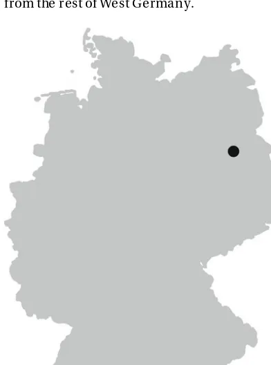
When using geospatial data to define features on the Earth, a Point geometry is generally used to represent an exact location, which could be a street address, or the location of a bank, volcano, or city, for instance. Figure 2-2 illustrates a Point geometry used to represent the location of Berlin with respect to a map of Germany. Berlin has a fascinating and complicated history, the city itself being politically divided for much of the twentieth century between West Berlin and East Berlin, a division that famously led to the erection of the Berlin Wall. Despite the fact that West Berlin was, to all intents and purposes, a part of West Germany, it lay in a region that, for 50 years following the Second World War, was proclaimed to be the German Democratic Republic (East Germany), and was entirely isolated from the rest of West Germany.

(29)

■Note Inasmuch as a Point geometry represents an infinitely small, singular location in space, it is impossible to truly illustrate it in a diagram. Throughout this book, Point geometries are represented as small black circles, as in Figure 2-2.

Defining a Point

A Point is defined by a pair of coordinate values, either an x-coordinate value and a y-coordinate value from a planar coordinate system, or a latitude and longitude coordinate value from a geographic coordinate system.

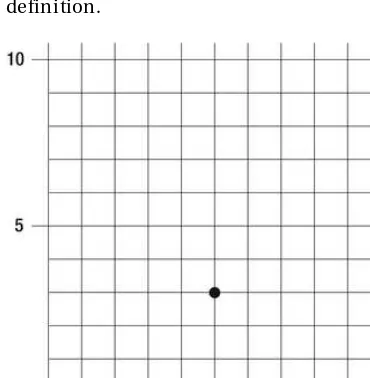
When expressed using the Well-Known Text (WKT) format, a Point located with coordinates x = 5 and y = 3 may be written as follows,

POINT(5 3)

The WKT representation begins with the POINT keyword followed by the relevant coordinate values, contained within round brackets. The coordinate values are separated by a space (not a comma, as you might initially expect). Figure 2-3 illustrates the Point geometry represented by this definition.

Figure 2-3. A Point located at POINT(5 3).

Defining a Point from geographic coordinates follows the same convention, but with one thing to watch out for: whereas in everyday language it is common to refer to coordinates of "latitude and longitude" (in that order), when you write geographic coordinates in WKT the longitude coordinate always comes first, then the latitude coordinate. The WKT syntax for a geography Point located at a latitude of 40° and longitude of 60° is therefore:

POINT(60 40)

(30)

Figure 2-4. A Point located at geographic coordinates POINT(60 40).

To help remember the correct order for geographic coordinates, try thinking of longitude as being equivalent to the x-coordinate, because longitude increases as you travel east around the world (until you cross the 180th meridian). Likewise, latitude is equivalent to the y-coordinate, with increasing latitude extending farther north. Because you list planar coordinates in (xy) order, the equivalent order for geographic coordinates is therefore (longitude latitude).

■Caution When defining geographic coordinates using WKT the longitude coordinate comes first, then the latitude coordinate.

Defining Points in 3- and 4-Dimensional Space

In addition to the x- and y- (or longitude and latitude) coordinates required to locate a Point on the surface of the Earth, the WKT syntax enables you to specify additional z-and m-coordinate values to position a point in four-dimensional space.

The z-coordinate is the height, or elevation, of a Point. Just as positions on the Earth's surface are measured with reference to a horizontal datum, the height of points above or below the surface are measured relative to a vertical datum. The z-coordinate may represent the height of a point above sea-level, the height above the underlying terrain, or the height above the reference ellipsoid, depending on which vertical datum is used.

(31)

route, the m-coordinate could be used to express the distance of how far along the route each point lay.

The WKT syntax for a Point containing z- and m-coordinates is as follows, POINT(x y z m)

Or, if using geographic coordinates:

POINT(longitude latitude z m)

However, you should be aware that, although SQL Server 2012 supports the creation, storage, and retrieval of z- and m-coordinate values, all of the inbuilt methods operate in 2D space only. The z and m values assigned to a Point instance will therefore not have any effect on the result of any

calculations performed on that instance.

For example, when calculating the distance between the Points located at (0 0 0) and (3 4 12), SQL Server calculates the result as 5 units (the square root of the sum of the difference in the x and y dimensions only), and not 13 (the square root of the sum of the difference in the x, y, and z

dimensions). You can, however, retrieve the z and m values associated with any instance and use them in your own calculations, as is demonstrated in a later chapter.

Characteristics of Points

All Point geometries share the following characteristics.

• A Point is zero-dimensional, which means that it has no length in any direction and there is no area contained within a Point.

• A Point has no boundary.

• The interior of a Point is the Point itself. Everything other than that Point is the exterior.

• Points are always classified as "simple" geometries.

LineStrings

Having established the ability to define individual Points, we can then create a series of two or more Points and draw the path segments that directly connect each one to the next in the series. This path defines a LineString.

Example LineString Usage

(32)

Figure 2-5. A LineString representing the route of the Orient Express railway.

Defining a LineString

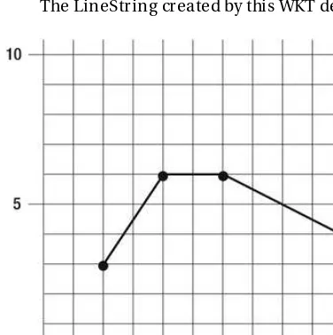
When expressed using the WKT format, the coordinate values of each Point are separated by a space, and a comma separates each Point from the next in the LineString, as follows.

LINESTRING(2 3, 4 6, 6 6, 10 4)

The LineString created by this WKT definition is illustrated in Figure 2-6.

(33)

■Note Some GIS systems make a distinction between a LineString and a Line. According to the Open Geospatial Consortium specification (a standard on which the spatial features of SQL Server 2012 are largely based), a Line connects exactly two Points, whereas a LineString may connect any number of Points. Because all Lines can be represented as LineStrings, of these two types SQL Server 2012 only implements the LineString geometry. If you need to define a table in which only Lines can be stored, you can do so by adding a CHECK constraint that calls the STNumPoints() method to test whether inserted LineString values contain only two points.

LineStrings created from geographic coordinates follow the same convention: the coordinates of each Point in the LineString are listed in longitude–latitude order (as they would be for an individual Point), and each Point in the LineString is separated by a comma.

Characteristics of LineStrings

All LineStrings are one-dimensional geometries: they have an associated length, but do not contain any area. This is the case even when the ends of the LineString are joined together to form a closed loop. LineStrings may be described as having the following additional characteristics.

• A simple LineString is one where the path drawn between the points of the LineString does not cross itself.

• A closed LineString is one that starts and ends at the same point. • A LineString that is both simple and closed is known as a ring.

• The interior of a LineString consists of all the points that lie on the path of the line. Be aware that, even when a LineString forms a closed ring, the interior of the LineString does not contain those points in the area enclosed by the ring. The interior of a LineString consists only of those points that lie on the LineString itself.

• The boundary of a LineString consists of the two points that lie at the start and end of the line. However, a closed LineString, in which the start and end points are the same, has no boundary.

• The exterior of a LineString consists of all those points that do not lie on the line. Different examples of LineString geometries are illustrated in Figure 2-7.

(34)

LineStrings and Self-Intersection

It is worth noting that, although the path of a nonsimple LineString may cross itself at one or more distinct points, it cannot retrace any continuous length of path already covered. Consider Figure 2-8, which illustrates the shape of a capital letter “T”:

Figure 2-8. A geometry in the shape of a capital letter T.

The shape illustrated in Figure 2-8 cannot be represented by a single LineString geometry, because doing so would necessarily involve retracing at least one section of the path twice. Instead, the appropriate type of geometry to represent this shape is a MultiLineString geometry, discussed later this chapter.

CircularStrings

As described in the previous section, LineStrings are formed by defining the path segments connecting a series of Points in order. The line segments that connect consecutive points are calculated by linear interpolation: each line segment represents the shortest direct route from one Point to the next in the LineString.

However, this is clearly not the only way to connect a series of Points. An alternative method would be to define a curve that connects each Point with a smooth line and gently changing gradient, rather than abrupt angular corners between segments typical of a LineString. The CircularString geometry, which is a new geometry type introduced in SQL Server 2012, provides one such curved line by using circular, rather than linear, interpolation between points. In other words, a CircularString is defined by the paths connecting a series of points in order, where the path segments connecting each pair of points is an arc formed from part of a circle.

Example CircularString Usage

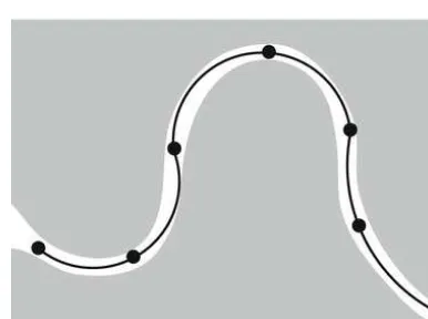
Every year, teams of rowers from Oxford University and Cambridge University compete in a boat race on the River Thames in West London. Starting from Putney Bridge, the race course follows the river upstream for slightly over four miles, ending just before Chiswick Bridge. The course is marked by three distinctive bends; the crew rowing on the north side of the river has the advantage in the first and third bends, whereas the crew rowing on the south side of the river has the advantage of being on the inside for the long second bend.

(35)

Figure 2-9. A CircularString geometry representing the course of the Oxford–Cambridge University boat race.

■Note Don't be misled by the name: a CircularString geometry does not have to form a complete circle (although it can); it merely means that the segments joining consecutive points are circular arcs rather than straight lines as in a LineString.

Defining a CircularString

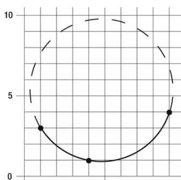
There are an infinite number of circular arcs that connect two Points. In order to specify which of these arcs should be created, every CircularString segment actually requires three points: the start and end points to be connected, and an additional anchor point that lies somewhere on the arc between those points. The CircularString will follow the edge of the only circle that passes through all three points.

The syntax for the Well-Known Text representation of a CircularString is as follows, CIRCULARSTRING (1 3, 4 1, 9 4)

(36)

Figure 2-10. CircularString defined by the circular interpolation of three points.

■Note The additional anchor point does not need to lie in the middle of the start and end points of a CircularString; it can be any point that lies on the circular arc between the start and end point.

Like LineStrings, CircularStrings can be created between a series of any number of consecutive points. Each segment implicitly starts at the endpoint of the previous curved segment. Each additional segment requires both an anchor point and an endpoint, therefore every valid CircularString contains an odd number of points, and must contain at least three points.

■Note A valid CircularString must have an odd number of points, greater than one.

WHEN IS A CIRCULARSTRING A STRAIGHT LINE?

One interesting point to note is that it is possible to specify a CircularString in which the anchor point lies exactly on the straight line between the start and end point. The circular arc created in such cases is a straight line, effectively joining all three points with the arc taken from a circle of infinite radius. The same result can also be achieved if the anchor point is exactly equal to either the start or end point.

The set of points contained by either a LineString or a "straight" CircularString are identical, which can be confirmed using SQL Server's STEquals() method as shown in the following code listing.

DECLARE @LineString geometry = 'LINESTRING(0 0, 8 6)';

(37)

DECLARE @CircularString2 geometry = 'CIRCULARSTRING(0 0, 0 0, 8 6)';

SELECT

@LineString.STEquals(@CircularString1), -- Returns 1 (true) @LineString.STEquals(@CircularString2); -- Returns 1 (true)

Characteristics of CircularStrings

CircularStrings, like LineStrings, inherit from the abstract Curve geometry type, and share many of the same characteristics.

• CircularStrings are one-dimensional geometries; they have an associated length, but do not contain any area.

• A simple CircularString is one where the path drawn between the points of the CircularString does not cross itself.

• A closed CircularString is one that starts and ends at the same point. • The interior of a CircularString consists of all the points that lie on the arc

segments.

• The boundary of a CircularString consists of the start and end points only, except in the case of a closed CircularString, which has no boundary.

• The exterior of a CircularString consists of all those points not on the path of the CircularString.

• Every CircularString must be defined by an odd number of points greater than one.

Drawing Complete Circles

To create a CircularString that forms a complete circle, you might expect that you would need to define only three points: one point used twice as both the start and end of the CircularString, and one other anchor point that lies somewhere on the perimeter of the circle. However, the problem with this definition is that it does not specify the orientation of the created circle; that is, beginning from the start point, does the path of the CircularString travel in a clockwise or anti-clockwise direction through the anchor point and back to where it started?

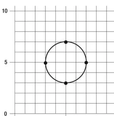
To avoid this ambiguity, in order to create a CircularString that forms a complete circle, five points are required. As with any closed LineString, the start and end points are the same. The remaining three points can be any other points that lie on the circle, listed in the desired order. The following Well-Known Text defines a clockwise circle with a radius of two units, centered about the point at (5 5):

CIRCULARSTRING(3 5, 5 7, 7 5, 5 3, 3 5)

(38)

Figure 2-11. Creating a circle using a CircularString geometry.

■Note In order to define a full circle, you must define a CircularString containing five points.

Choosing Between LineString and CircularString

Although LineString geometries can be used to approximate a curve by using a number of small segments, CircularStrings can generally do so more efficiently and with greater accuracy. However, even though the CircularString geometry may enable you to describe rounded features with greater precision, the LineString is better supported and more widely used in spatial applications. For this reason, you will probably find that many sources of spatial data still use LineStrings even in situations where CircularStrings may provide greater benefit.

You may also find that, when exporting your own data for use in third-party spatial applications, CircularStrings are not supported and you may have to convert your CircularStrings to LineStrings instead. Fortunately, SQL Server provides a method to do just this—STCurveToLine()—which is documented in Books Online at http://msdn.microsoft.com/en-us/library

/ff929272%28v=sql.110%29.aspx.

CompoundCurves

(39)

Example CompundCurve Usage

The Daytona International Speedway race track in Daytona Beach, Florida, is recognizable by its distinctive tri-oval shape, consisting of three straights and three smooth corners. This revolutionary circuit design, conceived by Bill France, founder of NASCAR, was created to maximize the angle of vision in which spectators could see cars both approaching and driving away from them.

Figure 2-12 illustrates a CompoundCurve representing the shape of the Daytona racing circuit, consisting of three CircularString segments and three LineString segments.

Figure 2-12. A CompundCurve representing the Daytona International Speedway racing circuit.

Defining a CompoundCurve

The Well-Known Text for a CompoundCurve geometry begins with the COMPOUNDCURVE keyword followed by a set of round brackets. Contained within the brackets are the individual LineString or CircularString segments that are joined together to form the compound curve.

Each CircularString or LineString segment in the CompoundCurve must begin at the point where the previous segment ended, so that the CompoundCurve defines a single continuous path. The coordinates of CircularString segments are preceded by the CIRCULARSTRING keyword, whereas LineString segments are not preceded by any keyword; they are simply a list of coordinates contained in round brackets.

The following code listing demonstrates the Well-Known Text representation of a

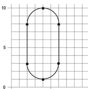
CompoundCurve geometry containing two LineString segments and two CircularString segments: COMPOUNDCURVE(

(2 3, 2 8),

CIRCULARSTRING(2 8, 4 10, 6 8), (6 8, 6 3),

CIRCULARSTRING(6 3, 4 1, 2 3) )

(40)

Figure 2-13. A CompoundCurve geometry.

Characteristics of CompoundCurves

CompoundCurves are constructed from one-dimensional LineStrings and CircularStrings, therefore CompoundCurves are themselves one-dimensional, and contain no area.

• A simple CompoundCurve is one that does not intersect itself.

• A closed CompoundCurve is one that starts and ends at the same point.

Polygons

A Polygon is a type of surface; that is, a Polygon is a two-dimensional geometry that contains an area of space. The outer extent of the area of space contained within a Polygon is defined by a closed LineString, called the exterior ring. In contrast to a simple closed LineString geometry, which only defines those points lying on the ring itself, the Polygon defined by a ring contains all of the points that lie either on the line itself, or contained in the area within the exterior ring.

Example Polygon Usage

(41)

Figure 2-14. A Polygon geometry representing the U.S. state of Texas.

Exterior and Interior Rings

Every Polygon must have exactly one external ring that defines the overall perimeter of the geometry. It may also contain one or more internal rings. Internal rings define areas of space contained within the external ring, but excluded from the Polygon. They can therefore be thought of as “holes” that have been cut out of the main geometry.

Figure 2-15 illustrates a Polygon geometry containing a hole. The Polygon in this case represents the country of South Africa, and the hole represents the fully enclosed country of Lesotho.

(42)

Defining a Polygon

The Well-Known Text for a Polygon begins with the POLYGON keyword, followed by a set of round brackets. Within these brackets, each ring of the Polygon is contained within its own set of brackets. The exterior ring, which defines the perimeter of the Polygon, is always the first ring to be listed. Following this, any interior rings are listed one after another, with each ring separated by a comma.

The following code listing demonstrates the WKT syntax for a rectangular Polygon, two units wide and six units high.

POLYGON((1 1, 3 1, 3 7, 1 7, 1 1))

And the following code listing demonstrates the WKT syntax for a triangular Polygon containing an interior ring.

POLYGON((10 1, 10 9, 4 9, 10 1), (9 4, 9 8, 6 8, 9 4))

These two Polygons are both illustrated in Figure 2-16.

Figure 2-16. Examples of Polygon geometries. (From left–right) A Polygon; a Polygon with an interior ring.

■ Note Because Polygons are constructed from rings, which are simple closed LineStrings, the coordinates of the start and end points of each Polygon ring must be the same.

Characteristics of Polygons

All Polygons share the following characteristics.

(43)

• Polygons are two-dimensional geometries; they have both an associated length and area.

• The length of a Polygon is measured as the sum of the lengths of all the rings of that Polygon (exterior and interior).

• The area of a Polygon is calculated as the area of space within the exterior ring, less the area contained within any interior rings.

CurvePolygons

The CurvePolygon, like the Polygon, is defined by one exterior ring and, optionally, one or more interior rings. Unlike the Polygon, however, in which each ring must be a simple closed LineString, each ring in a CurvePolygon can be any type of simple closed curve. Those curves can be LineStrings, CircularStrings, or CompoundCurves, so the rings that define the boundary of a CurvePolygon can have a mixture of straight and curved edges.

Example CurvePolygon Usage

Yankee Stadium, built in 1923 in New York City, hosted over 6581 home games of the New York Yankees baseball team in its 85-year history, prior to its closure in 2008 (the team now plays in a new stadium, also named “Yankee Stadium,” constructed a short distance away from the site of the original Yankee Stadium). It was the first three-tiered sports facility to be built in the United States, and one of the first to be officially named a stadium (as opposed to a traditional baseball park, or field).

The large stadium was designed to be a multipurpose facility that could accommodate baseball, football, and track and field events, and the smooth-cornered, irregularly sided shape of the stadium can be be modeled as a CurvePolygon whose exterior ring contains four CircularString segments and four LineString segments, as illustrated in Figure 2-17.

(44)

Defining a CurvePolygon

The WKT representation of a CurvePolygon follows the same general syntax as that for a Polygon. However, because the CurvePolygon allows rings to be defined as LineStrings, CircularStrings, or CompoundCurves, you must specify which kind of curve is used for each ring.

The LineString is considered to be the “default” curve type, and linear rings do not need to be explicitly preceded by the LINESTRING keyword. In the following code listing, a CurvePolygon is defined by a linear ring between five points:

CURVEPOLYGON((4 2, 8 2, 8 6, 4 6, 4 2))

The result, shown in Figure 2-18, is a square of width and height 2 units, exactly the same as would have been created using the following Polygon geometry.

POLYGON((4 2, 8 2, 8 6, 4 6, 4 2))

Figure 2-18. A CurvePolygon with a LineString exterior ring.

In the following code listing, the exterior ring of the CurvePolygon is instead defined using a CircularString geometry between the same set of points.

CURVEPOLYGON(CIRCULARSTRING(4 2, 8 2, 8 6, 4 6, 4 2))