M. Imani, H. Ghassemian
Faculty of Electrical and Computer Engineering, Tarbiat Modares University, Tehran, Iran
[email protected]
[email protected]
hyperspectral data, limited training samples, non"parametric classifier
One of the most important and challenging problems in supervised classification of high dimensional data is limited
available training samples. Using the parametric classifiers is not appropriate in this condition. Thus a new simple non"
parametric supervised classifier based boundary samples of each class is proposed in this paper that need no statistic
parameter for classification. Accuracy and reliability of this classifier is compared whit other non"parametric classifiers
such as Parallelepiped (box), K nearest neighbours (KNN), Artifical Neural network (ANN) and SVM and also a
parametric classifier that use only first order statistic, Minimum Euclidean Distance (MED), for different four datasets,
AVARIS data, Pavia University, Pavia center and Salinas data. The results of experiments show that proposed classifier
in despite of simplicity has appropriate and reasonable efficiency.
Obtaining more details for discrimination between classes has become possible in recently years using hyperspectral images. Supervised classification of high dimensional data need to more training samples that is not enough available. In many hyperspectral images, spectral signature of different classes are similar and then using only first order statistic (mean vector) is not efficient for classification of data. Also using of second order statistic that means covariance matrix is not possible. Because the estimation of covariance matrix using limited training samples is inaccurate and singularity problem is occurred. So, when we involve in high dimensional data and the size of training set is small, the best solution for classification is non"parametric classifiers such as SVM (Li, 2012, Mianji, 2011, Mũnoz"Marí, 2010, Marconcini, 2009), Artifical Neural network (ANN) (Ratle , 2010, Lin, 2002, Del Frate , 2007), k" NN (Li, 2010, Yang , 2010), and Parallelepiped (box) (Meng , 2011) . The best known classifier for high dimensional data and limited training samples is support vector machine. In SVM a separating hyperplane whit maximal margin is found for discrimination of two classes. Training vectors are mapped into a higher dimensional space by a mapping function. The burden of computational in SVM is relatively high. A common criticism of neural networks is that they require a large diversity of training samples in order to capture the underlying structure that allows it to generalize to new cases. KNN is a non" parametric classifier based on closest training examples in the feature space. is a constant that defined by user and the choice of it depends upon the data generally .then user has to select the appropriate value for parameter k for each new data to achieve the best efficiency in classification. Box classifier is quick to run but not very accurate as the parallelepipeds are formed based on their max and min sample values that may not be representative of a class. The sample may not lie inside any of
the regions defined by the parallelepipeds or lie inside two or more overlapping parallelepipeds.
A new simple non"parametric supervised classifier based boundary samples of each class is proposed in this paper and compared whit other non"parametric classifiers in different datasets. The reminder of this paper is organized as follows: in section 2, we represent the proposed classifier and experimental results are given in section 3. This paper is concluded in section 4.
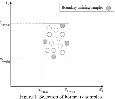
The first step in the proposed algorithm is the finding of boundary samples across training samples in each class. Each training sample that at least one of values of their features is minimum or maximum is considered as boundary sample in our definition. In the second step, the distance of test sample from boundary samples of each class is calculated and boundary sample that its distance from test sample is minimum is selected as deputy of it class. In the third step, label of class that its deputy is nearest to test sample is assigned to it test pixel. and that are dimensional vectors, denote boundary sample of class and test sample respectively. Also the number of training samples of class and the number of classes are and respectively. The label of test sample is calculated as follows:
= arg min ,…, ( − ) (1)
The used distance in above equations is Euclidean distance that defined as follows:
( , ) = ( − ) ( − ) (2)
Where ( ) denote transpose of vector . Figure 1 shows how to select boundary samples in each class in two dimensions. The proposed classifier for especial case of two classes in two
Figure 1. Selection of boundary samples
dimensions is represented in Figure 2. Note that the proposed classifier is equivalent to the KNN classifier whit K=1 when all training samples are considered as boundary samples.
! "# $! ! %&! '( ) *% +'"
Four different datasets are used for experiments in this section. The first hyperspectral data is Airborne Visible/Infrared Imaging Spectrometer (AVIRIS) Indian pines image. This image has spatial dimension 145×145 and containes 16 classes that most of which are different types of crops. The AVIRIS sensor generates 220 bands that we reduced the number of them to 190 by removing 30 absorption and noisy bands. The second and third used datasets (university of Pavia and center of Pavia) are acquired by Reflective Optics System Imaging Spectrometer (ROSIS). The number of spectral bands is 103 for university of Pavia and 102 for center of Pavia. University of Pavia is a 610×340 pixels image and center of Pavia is consist of 1096×715 pixels. Both of these urban images contain 9 classes. Salinas scene that collected by the 224 band AVIRIS sensor over Salinas valley, California, is the fourth used dataset that 20 absorption bands of it is discarded and 204 reminded bands are used. Salinas image is a 512×217 image with 16 classes. We randomly choose just 10 training samples of the labeled samples per class for training and use the rest of samples for testing in all experiments.
The used measures for comparison of classifiers are average accuracy and average reliability. Accuracy and reliability for each class defined as follows: accuracy is the number of test samples that are correctly classified divided to the total test samples and reliability is number of test samples that are correctly classified divided to the total samples that are labeled as this class. The average accuracy and average reliability are the mean of the class accuracies and reliabilities respectively. The represented results are average of acquired values after three times iterations. Used artifical neural network in our experiments is back propagation network with 30 neurons in hidden layers. The parameter k in k"NN classifier in each datasets is selected such that the best posible acccuracy is acquired.
Figure 2. The representation of proposed classifier
,-!&+.!" * ! %*
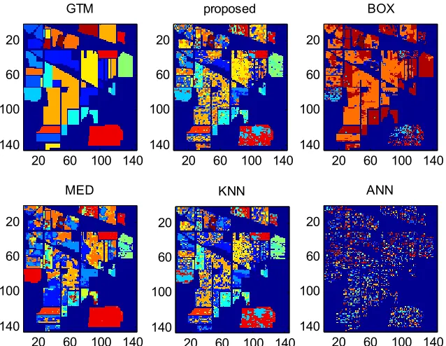
The new non"parametric classifier is evaluated in this section. We compare it with the other non"parametric classifiers such as BOX, KNN, ANN and SVM classifiers. Also MED classifier that used only the first order statistic parameter is compared with non"parametric classifiers. It is worth note that a parametric classifier such as maximum likelihood (ML) is not involve in comparison because the minimum number needed training samples for training of this classifier is equal to the number of features add one while we discuss about limited training samples. The results of experiments are represented in this section. Figure 3 show the comparison of classifiers from the viewpoint of accuracy and reliability for Indiana, university of Pavia, center of Pavia and Salinas datasets. The obtained classification maps are shown in Figures 4"7. The Summary of comparison of accuracy and reliability of classifiers for different images are given in Tables 1 and 2 respectively. The results of experiments show that the best classifiers for hyperspectral images with limited training samples are SVM, proposed and KNN classifiers respectively. The most accuracy and reliability are acquired by SVM that is a powerful tool for classification of high dimensional data whit small training sample size. But the computational complexity and thus the cost of this learning machine is relative high. After SVM, our proposed classifier that uses a simple algorithm for classification has the best results with average 3.86% difference in accuracy and 4.71% in reliability that seems reasonable and appropriate.
Figure 3. Comparison of accuracy and reliability of Indiana, university of Pavia, center of Pavia and Salinas datasets
Figure 4. Ground Truth Map (GTM) and classification maps for Indiana Image
! !
""# "$ % & % !$
' ( !$ ) ( ! !
""# "$ % & % !$
*
% " ! !
""# "$ % & % !$ *
+ ! ) ( ! !
""# "$ % & % !$
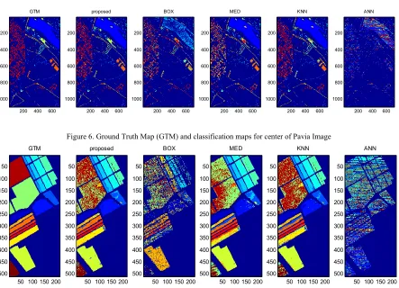
Figure 5. Ground Truth Map (GTM) and classification maps for university of Pavia Image
Figure 6. Ground Truth Map (GTM) and classification maps for center of Pavia Image
Figure 7. Ground Truth Map (GTM) and classification maps for Salinas Image
Table 1. Summary of comparison of accuracy of classifiers for different images Average accuracy Indian
Pines
University of Pavia
Center of Pavia
Salinas scene
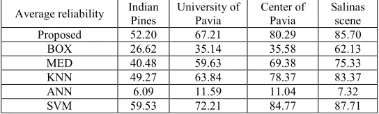
Proposed 66.00 73.55 84.26 87.88
BOX 21.73 39.23 41.28 48.50
MED 50.13 66.56 73.29 77.02
KNN 60.64 72.38 81.96 85.20
ANN 6.30 11.30 11.12 6.97
SVM 71.69 76.93 88.17 90.35
Table 2. Summary of comparison of reliability of classifiers for different images
/
In this paper, a new simple non"parametric classifier is proposed that is based on boundary samples. The obtained accuracy and reliability of this classifier is relative close to SVM that known as the best classifier for high dimensional data with limited training samples.
Del Frate F. , 2007, Pacifici F. , Schiavon G. , and C. Solimini. Use of Neural Networks for Automatic Classification From High"Resolution Images.
., 45(4), pp. 800 – 809 (April 2007).
Li C.H., 2012, Kuo B."C. , Lin C."T., and Huang C."S. A Spatial–Contextual Support Vector Machine for Remotely Sensed Image Classification.
, 50(3), pp. 784 " 799 (March 2012).
Li M., 2010, Crawford M.M. , Jinwen T. , “Local Manifold Learning"Based k"Nearest"Neighbor for Hyperspectral Image Classification ,”
., 48(11), pp. 4099 " 4109 (Nov. 2010).
Lin J."S., 2002, Liu S."H. Classification of multispectral images based on a fuzzy"possibilistic neural network.
! , 32(4), pp. 499 " 506 (Nov. 2002).
Marconcini M., 2009, Camps"Vails G. , and Bruzzone L. A Composite Semisupervised SVM for Classification of
Hyperspectral Images.
" , 6(2), pp. 234 " 238 (April 2009).
Meng W., 2011, Lianpeng Z. , Shichen C. , Weiwei M., and Yangyang G. The analysis about factors influencing the supervised classification accuracy for vegetation hyperspectral remote sensing imagery. # $
, 3, pp. 1685 – 1689 (Oct. 2011).
Mianji F.A.,2011 and Ye Zhang. SVM"Based Unmixing" to"Classification Conversion for Hyperspectral Abundance
Quantification. ,
49(11), pp. 4318 – 4327 (Nov. 2011).
Mũnoz"Marí J., 2010, Bovolo F., Gomez"Chova L. , Bruzzone L. , and Camp"Valls G. Semisupervised One" Class Support Vector Machines for Classification of Remote Sensing Data.
, 48(8), pp. 3188 " 3197 (Aug. 2010).
Ratle F., 2010, Camps"Valls G., and Weston J. Semisupervised Neural Networks for Efficient Hyperspectral Image Classification.
, 48(5), pp. 2271 " 2282 (May 2010).
Yang J."M., 2010 Yu P."T. , and Kuo B."C. A Nonparametric Feature Extraction and Its Application to Nearest Neighbor Classification for Hyperspectral Image
Data . ., 48(3), pp.