SPATIOTEMPORAL EVOLUTION OF THE IMBALANCED REGIONAL
DEVELOPMENT IN MAINLAND CHINA USING DMSP-OLS DATA
Kai Chena, Tao Jia a, * a
School of Remote Sensing and Information Engineering, Wuhan University, Wuhan, China - [email protected], [email protected]
Commission IV, WG IV/3
KEY WORDS: DMSP-OLS
,
Correlation Analysis, Regional Development Center,
Imbalanced RegionalDevelopment
,
Regional Development GiniABSTRACT:
The Defense Meteorological Satellite Programs Operational Linescan System (DMSP-OLS) nighttime lights imagery has been widely used to monitor economic activities and regional development in recent decades. In this paper, we firstly processed the nighttime light imageries of the Mainland China from 1992 to 2013 due to the radiation or geometric errors. Secondly, by dividing the Mainland China into seven regions, we found high correlation between the sum light values and GDP of each region. Thirdly, we extracted the economic centers of each region based on their nighttime light images. Through the analysis, we found the distribution of these economic centers was relatively concentrated and the migration of these economic centers showed certain directional trend or circuitous changes, which suggested the imbalanced socio-economic development of each region. Then, we calculated the Regional Development Gini of each region using the nighttime light data, which indicated that social-economic development in South China presents great imbalance while it is relatively balanced in Southwest China. This study would benefit the macroeconomic control to regional economic development and the introduction of appropriate economic policies from the national level.
1. INTRODUCTION
The nighttime light (NTL) time-series image data from DMSP-OLS reveals all the changes occurred in every country over the last 20 years. Recent studies showed that these data were highly correlated with population, economic growth, foreign investment, war and economic decline(Changjiang Daily,2012.), hence they have a wide range of
applications
(
Elvidge, C. D. et al.,2009; Liu, Z. et al.,2012).He, et al. studied the urbanization process of Bohai Rim in the 1990s using NTL data and developed three basic urban models of polygon-urbanization, line-urbanization and point-urbanization(Chunyang et al.,2003). The findings from a recent study lend support to the hypothesis that night-time light can be a useful source for monitoring humanitarian crises such as that unfolding in Syria(Li, X.et al.,2014). Sutton used DMSP-OLS data as a scale-adjusted measure of “Urban sprawl” to study about how the dynamics of “Urban Sprawl” are changing (Sutton, P. C. ,2003). Muller and Morley provided the first detailed examination of night-time light characteristics with respect to local economic activity and highlight issues in their findings(Doll, C. N. H.et al.,2006).Imhoff, M. L.et al. (Imhoff, M. L.et al.2004) used data from DMSP-OLS and a terrestrial carbon model to quantify the impact of urbanization on the carbon cycle and food production in the US as a result of reduced net primary productivity.
Therefore, this study aimed to explore the imbalance of regional development using high temporal frequency NTL data from two perspectives of economic centre migration and Regional Development Gini. Specifically, we firstly calibrated the NTL data and conducted a correlation analysis between the total amount of GDP and sum light values of seven regions. The good fitting result indicates that the NTL data can be used to reflect the regional economic and development situation. Then, we calculated the regional development centers of Mainland China from the DMSP-OLS data and took the year in 1993, 2003, and 2013 to explore the dynamic migration of centers in each region. Moreover, we calculated the Regional Development Gini derived from DMSP-OLS data of each region and analyse their dynamic change, based on which we further explored the imbalance of regional economic development of each region.
2. DATA
intercalibration and inter-annual adjustment.
Figure 1. Sum light values of the Mainland China before intercalibration(a) and after intercalibration (b)
2.1 Intercalibration
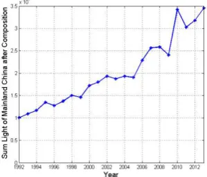
Due to the influence of the radiation error, the original DMSP-OLS data we got for the same year from different satellites usually contradicts each other, which may interfere with our subsequent work. Figure 1(a) is the time-series graph of DMSP-OLS sum light values for Mainland China from year 1992 to 2013. As we can see, there is DMSP-OLS data collecting by different satellite for most years and its sum light values shows great discrepancy, which need a stable and reliable intercalibrating method to minimize this discrepancy. Using the method proposed by Elvidge et al., we assume Sicily, Italy to be a region with no change in nighttime light from 1994 to 2008. The 1999 annual image composite collected by DMSP satellite F12 is selected as a reference image because data from this annual image composite have the largest DN values. ( Zhao, N.,et al.,2014)A group of second-order regression functions was developed by adjusting DN values of pixels in Sicily of candidate images to the match DN values of pixels in Sicily in the reference image. The second-order functions we got in Table 1 are then used to calibrate their corresponding nighttime light images. Figure 1(b) shows the time-series graph of DMSP-OLS sum light values for Mainland China after our intercalibration. What we can see is our intercalibration has significantly improved the discrepancy in DMSP-OLS data.
Figure 1. Sum light values of the Mainland China before intercalibration(a) and after intercalibration (b)
DNcalibration=C0+C1*DN+C2*DN2 Satellite Year C0 C1 C2 R2
F10 1992 1.2019 0.5761 0.0048 0.9299 F10 1993 1.3462 0.5168 0.006 0.9502 F10 1994 0.7319 0.5703 0.0057 0.9514 F12 1994 0.3928 0.8327 0.0016 0.9415 F12 1995 0.7325 0.7361 0.0033 0.9498 F12 1996 0.4205 0.715 0.0033 0.9567 F12 1997 0.7194 0.8155 0.0018 0.9514 F12 1998 0.5833 0.9085 0.0011 0.9693
F12 1999 0 1 0 1
F14 1997 0.882 0.4759 0.006 0.9351 F14 1998 0.5538 0.4904 0.0068 0.9761 F14 1999 0.8329 0.5399 0.006 0.9779 F14 2000 0.5026 0.6105 0.0051 0.9529 F14 2001 0.7489 0.6421 0.0046 0.9627 F14 2002 0.2091 0.7508 0.0032 0.949 F14 2003 0.6544 0.6889 0.0038 0.9611
Satellite Year C0 C1 C2 R2 F15 2000 1.2194 0.8792 0.0013 0.9539 F15 2001 0.9965 0.8899 0.0008 0.968 F15 2002 0.7833 0.962 -0.0005 0.9743 F15 2003 0.9093 0.5349 0.0055 0.951 F15 2004 0.5385 0.6249 0.0048 0.9654 F15 2005 0.8048 0.6653 0.0039 0.9538 F15 2006 0.5778 0.6714 0.0037 0.9578 F15 2007 0.3381 0.6314 0.0039 0.9351 F16 2004 0.7003 0.7726 0.0027 0.9397 F16 2005 1.0298 0.5764 0.0052 0.9599 F16 2006 0.5901 0.8139 0.0014 0.9473 F16 2007 0.5 0.9995 -0.0006 0.9662 F16 2008 0.4284 0.9376 0.0005 0.9625 F16 2009 0.0704 0.8583 0.0016 0.9366 F18 2010 0.5666 1.357 -0.0067 0.9091 F18 2011 0.0524 1.1621 -0.0027 0.9448 F18 2012 0.2388 1.2566 -0.0044 0.9581 F18 2013 0.0287 1.2011 -0.003 0.9564 Table 1. The second-order intercalibration functions
and parameters
2.2 Inter-annual Adjustment
After our intercalibration, there is still some discrepancy in data from different satellites for the same year, which need a method to adjust the data in order to only reserve one valid data for the same year. So we adopted the following inter-annual adjustment method. If the pixel value of the same place in DMSP-OLS nighttime light images collected by two satellites for the same year are both the nonzero value, the two pixels are considered stable pixel and the mean value of the two pixels are taken as the result pixel value. If one of the two pixels has a value of zero, the pixels are considered unstable pixels and the result pixel value is 0. We describe our approach as Eq. (1), in which
��
(��,�),
��
(��,�) refers to the DNvalues of pixel i in year n collected by different satellites. Using this method, we accomplished the inter-annual adjustment for the DMSP-OLS nighttime light images of Mainland China which greatly improves the reliability of our data. Figure 2 shows the time-series graph of DMSP-OLS sum light values for Mainland China after our inter-annual adjustment.
Figure 2. Sum light values of the Mainland China after inter-annual adjustment
��(�,�) =� 0,��(�,�)
� = 0 ���� (��,�)= 0
(��(��,�)+��(��,�))/2,��ℎ������ (1)
3. ANALYSIS AND RESULTS
3.1 The correlation analysis of sum light values with GDP
To verify the feasibility of using sum light values of each region as a proxy for investigating its economic development, we adopted GDP and population data of 31 provinces in Mainland China from year 1992 to 2013 from National Bureau of Statistics of the People’s Republic of China, then we conducted the correlation analysis between sum light values and GDP for eseven regions (Central China, North China, South China, East China, Northeast China, Southwest China and Northwest China) and Mainland China. The result is shown in Table 2.
As we can see, the R-square value of correlation analysis between sum light values and GDP for Mainland China is 0.92. Its fitting result is superior to that in the seven regions, the reasons for which are manifold. Some come from the error of DMSP-OLS data, others come from the instability of GDP growth. In spite of that, the R-square values of correlation analysis between sum light values and GDP for seven regions are all greater than 0.8. This finding is consistent with other findings in the literature(He, C., et al.,2006; Mellander,C.et al.,2015; Xu, H.et al.,2007),which suggested the feasibility of using sum light values of each region as a proxy for investigating its economic development.
Regions in Mainland China R2
Mainland China 0.92(**)
Central China 0.85 (**)
North China 0.91(**)
South China 0.87(**)
East China 0.92(**)
Northeast China 0.87(**)
Southwest China 0.87(**)
Northwest China 0.92(**)
Table 2. The square of correlation coefficient (** indicates 1% significant level)
3.2 The evolution of the regional development centers in Mainland China
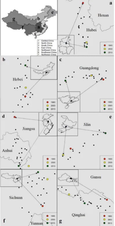
After verifying the highly correlation between DMSP-OLS data and GDP, we extracted the time-series image for seven regions of Mainland China from DMSP-OLS NTL image data which has been processed by intercalibration and inter-annual adjustment. Then we calculated the regional development centers of each region in Mainland China using Eq. (2) based on these DMSP-OLS data, where DN refers to digital number of the DMSP-OLS image pixel and X or Y refers to geographic coordinate. The regional development centers for seven regions of Mainland China we got are shown in
Figure 4. For the seven regions, we all selected year 1993, 2003,2013 to explore the evolution of the regional development centers.
����=∑ ���∗ ��/∑ ���
�=∑ ���∗ ��/∑ ��� (2)
Central China includes Henan, Hubei, Hunan and Jiangxi Province. As we can see from Figure 3(a), the centers from year 1993 to 2013 are all distributed in the north of Hubei Province and on the north of Hunan and Jiangxi Province. Henan lies in the north of these centers. As for GDP, we found the GDP growth of 1993-2003 and 2003-2013 in Henan Province are 313.67 % and 368.73% respectively. But the GDP growth of Hubei, Hunan, and Jiangxi in 1993-2013 are 258.83%, 274.38% and 288.28% respectively and in 2003-2013 are 421.12 %, 428.36% and 413.29% respectively. It is obvious that the total GDP growth in southern three provinces is higher than that in Henan Province, which causes the continued southward movement of regional development centers in Central China from year 1993 to 2013. Moreover, the population growth of Henan, Hubei, Hunan and Jiangxi are -2.63%, 2.01%, 0.42% and 6.29%, which also explains the continued southward movement of the centers from the other side.
North China includes Beijing, Tianjin, Hebei, Shanxi and Inner Mongolia. From Figure 3(b), we can see these centers are all distributed in Hebei Province. And the center of year 2003 has a northward movement relative to year 1993, more close to Beijing. As for GDP, we found the GDP growth of Beijing is 465.01%, which is much higher than that of Hebei and Shanxi with a growth of 309.34 % and 319.63% respectively. In 2003-2013, Inner Mongolia in the northern part of North China gets a GDP growth of 608.28%, far exceeding that of Hebei and Shanxi, whith a GDP growth of 310.95% and 343.58% respectively, which explained the substantial northward movement of regional development centers in North China in 2003 to 2013.
South China includes Guangdong, Guangxi and Hainan. Guangdong is an economic giant in Mainland China for a long time. As we can see from Figure 3(c), the centers of South China are distributed in an east-west narrow belt in Guangdong. Besides, the center of year 2003 has a westward movement relative to year 1993, and in 2003-2013 there is another substantial westward movement with almost negligible south-north movement. The continued westward movement of centers in 1993-2013 stems from the greatly economy development of Guangxi in these years. Especially in 2003-2013, the GDP growth of Guangxi is 412.21% which is higher than that of Guangdong (294.30%). It shows the economic attractiveness of Guangxi is increasing year by year.
East China includes Shandong, Jiangsu, Anhui, Zhejing, Fujian and Shanghai, in which Shanghai is one of the economic centers in Mainland China and the international metropolis. From Figure 4(d), we can see the centers of East China are distributed in a south-north narrow belt in the junction of Anhui and Jiangsu. In 1993 to 2003, the provinces in southern part of East China, Zhejiang and Fujian get a GDP growth of 403.92% and 347.29% while southern part province, Shandong, Jiangsu and Anhui get a GDP growth of 335.98% 、 315.02% and 278.26% respectively, which are relatively low. The economic growth advantage in southern province causes the southward movement in 1993-2003.While the center of year 2013 appears a westward movement relative to year 2003, at the same time the GDP growth of Shanghai in the east decrease to 225.92% relative to that of Anhui (390.16%), which indicates the economic growth of Shanghai is slowing down and the economy of East China is changing into a relatively balanced development.
Northeast China consists of Liaoning, Jilin and Heilongjiang. As we can see from Figure 3(e), its regional development centers are distributed in a northeast-southwest belt in Jilin which is on the south of Heilongjiang and north of Liaoning. The center of 2003 has a minor southwestward movement relative to year 1993 while in 2003-2013, there is a northeastward movement in these centers. As for GDP data, we did not find some corresponding factors in Heilongjiang and Liaoning which can cause the migration of these centers. But the central part province, Jilin gets a GDP growth of 270.46% and 390.08% in 1993-2003 and 2003-2013 respectively, which has a dominant advantage relative to the other
two provinces. We guess this may have something to do with the evolution of regional centers in Northeast China. And there may exist other more complex economic or population factors, but we cannot get a clear conclusion about this.
Southwest China includes Sichuan, Yunnan, Guizhou, Xizang and Chongqing. As we can see from Figure 3(f), the regional development centers are distributed in the south part of Sichuan. In 1993-2003, the southern part provinces, Yunnan and Guizhou get a GDP growth of 226.33% and 241.48% while the northern part provinces, Sichuan and Chongqing get a higher GDP growth of 258.97% and 319.98% (Xizang is negligible because of its small amounts of GDP), which leads to the large northward movement in 1993-2003. As for the center in year 2013, it has a northwestward movement relative to year 2003, obviously farther from Guizhou. We further found the population of Guizhou has a negative growth (-9.51%) while the population growth of Xizang is 14.71%. So we consider it is population factor that leads to the evolution of its Regional Development centers in 2003-2013.
The last one is Northwest China, including Ningxia, Xinjiang, Qinghai, Shaanxi and Gansu, which are always in a disadvantaged position due to the natural and historical factors. As is shown in Figure 3(g), the regional development centers are distributed in the junction of Qinghai and Gansu. In 1993-2003, the population growth of Shaanxi and Gansu are 4.53% and 4.06% while Xinjiang's population grows at a high rate of 20.5%, which causes that the centers have a substantial westward movement, more close to Xinjiang. And the center in 2013 has a southeastward movement relative to 2003. As for GDP, we found the southeastern part provinces, Ningxia and Shaanxi get a GDP growth of 478.76% and 526.24%, while the northwestern part, Xinjiang gets a GDP growth of 347.63%. Thus it can be seen Xinjiang's economic growth stemming from energy is slowing down
(
Xiaobei Mao, 2015), and the regional development centers in Northwest China is moving back to Southeast.3.3 The evolution of the imbalance of regional development in Mainland China
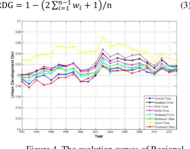
In this section, we further calculated the Regional Development Gini (RDG) which can reflect the imbalance of regional development using Eq. (3). Considering regional light values as regional development level, we ordered the pixels in the region from low to high according to their values and divided into equal numbers of n groups. In Eq. (3),
�
� refers to the proportion of accumulated DN values from group 1 to group i. After calculating RDG for each region, we show the evolution curve of each region and Mainland China from 1992 to 2013 in Figure 5. The higher the Regional Development Gini, the more imbalanced development the region(Cauwels, P.et al.,2014).fluctuation, which has a lot to do with the national macro-control. Moreover, these RDG curves all reach the maxima in year 2003 and reach the minima in year 2010. In 2002, high-tech industry and fast-growing industries such as automotive industry, electronic communications were developing swiftly and violently, densely distributed in big cities( Hongxia Cui, 2003), which brought about the imbalance of regional development in 2003. In 2010, the Nation adopted a proactive fiscal policy and an appropriately easy monetary policy and the State Council implemented plans to restructure and reinvigorate key industries(China Mining, 2011.),ensuring the uniform growth of regional economy and the balanced development of regional industry, which led to a balance of regional development in 2010. Besides, on average, we found South China presents the highest RDG value while Central China and Southwest China gets relatively low values. It is our assumption that Guangdong, the economic giant, might cause the high imbalance development in South China.
RDG = 1− �2∑�−1�=1��+ 1�/n (3)
Figure 4. The evolution curves of Regional Development Gini (RDG)
4. CONCLUSION
In this study, we explored the evolution of imbalanced regional development in Mainland China using DMSP-OLS data. We explored the distribution and migration of regional centres, which were well explained from the GDP and population factors. We further investigated the imbalance of regional development, and the conclusion is the level of regional development in South China presents great imbalance while Southwest China presents a relatively balanced regional development.
However, we didn’t study the quantitative relationship between the migration of these regional centers and the imbalance of regional development, which points out our future research. In general, this study would benefit the macroeconomic control to regional economic development and the introduction of appropriate economic policies from the national level.
ACKNOWLEDGMENTS
I owe my great debt of gratitude to Chu Ma, Yuqian Li, Qi Li and Xuesong Yu, who have given me his constant help and offered me invaluable advice and informative suggestions. My sincere thanks also go to
the anonymous referees for their careful work and thoughtful suggestions which will help me improve this paper substantially.
REFERENCES
Cauwels, P., Pestalozzi, N., & Sornette, D.,2014. Dynamics and spatial distribution of global nighttime lights. Epj Data Science, 3(1), 2.
Changjiang Daily ,2012. Report on the bc. tech-ex “The synchronous growth of light and GDP”, http://bc.tech-ex.com/technology/bccenter/2012/27 096.html(7 Dec.2012).
China Mining, 2011. Report on Chinamining.com “Summary of China's macroeconomic policies in 2010”,http://www.chinamining.com.cn/news/listne ws.asp?siteid=316563&ClassId=154 (3 Jan. 2011 ) Chunyang, Jinggang, CHEN, Jing, Peijun, & CHEN,
et al.,2006. The urbanization process of bohai rim in the 1990s by using dmsp/ols data. Journal of Geographical Sciences,16(2), 174-182.
Doll, C. N. H., Muller, J. P., & Morley, J. G. ,2006. Mapping regional economic activity from night-time light satellite imagery. Ecological Economics, 57(1), 75-92.
Elvidge, C. D., Ziskin, D., Baugh, K. E., Tuttle, B. T., Ghosh, T., & Pack, D. W., et al. ,2009. A fifteen year record of global natural gas flaring derived from satellite data. Energies, 2(3), 595-622. He, C., et al. ,2006.Restoring urbanization process in
China in the 1990s by using non-radiance calibrated DMSP/OLS nighttime light imagery and statistical data. CHINESE SCIENCE BULLETIN, 2006. 51(13): p. 1614-1620.
Hongxia Cui ,2003. The economic situation and policy analysis in 2003.
Imhoff, M. L., Bounoua, L., Defries, R., Lawrence, W. T., Stutzer, D., & Tucker, C. J., et al.,2004. The consequences of urban land transformation on net primary productivity in the united states. Remote Sensing of Environment, 89(4), 434-443.
Mellander, C., Lobo, J., Stolarick, K., & Matheson, Z., 2015. Night-time light data: a good proxy measure for economic activity?. Working Paper, 10(10), e0139779.
Li, X., & Li, D.,2014. Can night-time light images play a role in evaluating the syrian crisis?. International Journal of Remote Sensing, 35(18), 6648-6661.
Liu, Z., He, C., Zhang, Q., Huang, Q., & Yang, Y.,2012. Extracting the dynamics of urban expansion in china using dmsp-ols nighttime light data from 1992 to 2008. Landscape & Urban Planning, 106(1), 62-72.
Sutton, P. C. ,2003. A scale-adjusted measure of “urban sprawl” using nighttime satellite imagery. Remote Sensing of Environment, 86(3), 353-369. Xiaobei Mao, 2015. Report on the Cien News
“Diversified development of energy economy in Xinjiang”,http://www.cien.com.cn/content-126751. html(24 Sep. 2015)
Zhao, N., Zhou, Y., & Samson, E. L. ,2014. Correcting incompatible dn values and geometric errors in nighttime lights time-series images. IEEE