www.elsevier.nlrlocaterisprsjprs
A framework for the modelling of uncertainty between remote
sensing and geographic information systems
Mark Gahegan
a,), Manfred Ehlers
ba
Department of Geography, The PennsylÕania State UniÕersity, UniÕersity Park, PA 16802, USA
b
Institute for EnÕironmental Sciences, UniÕersity of Vechta, Germany
Received 29 March 1999; accepted 4 March 2000
Abstract
Ž .
This paper addresses the modelling of uncertainty in an integrated geographic information system GIS , specifically focused on the fusion of activities between GIS and remote sensing. As data is abstracted from its ‘raw’ form to the higher representations used by GIS, it passes through a number of different conceptual data models via a series of transformations. Each model and each transformation process contributes to the overall uncertainty present within the data. The issues that this paper addresses are threefold. Firstly, a description of various models of geographic space is given in terms of the inherent uncertainty characteristics that apply; this is then worked into a simple formalism. Secondly, the various transformation processes that are used to form geographic classes or objects from image data are described, and their effects on the uncertainty properties of data are stated. Thirdly, using the formalism to describe the transformation processes, a framework for the propagation of uncertainty through an integrated GIS is derived. By way of a summary, a table describing sources of accumulated uncertainty across four underlying models of geographic space is derived.q2000 Elsevier Science
B.V. All rights reserved.
Keywords: uncertainty; GIS integration; data modelling; transformation description
1. Introduction
Good science requires statements of accuracy by which the reliability of results can be understood and communicated. Where accuracy is known objec-tively, then it can be expressed as error, where it is
Ž
not, the term uncertainty applies Hunter and Good-.
child, 1993 . Thus, uncertainty covers a broader range of doubt or inconsistency, and in the context of this paper, includes error as a component. The
under-)
Corresponding author. Tel.:q1-814-865-2612; fax:q 1-814-863-7943 http:rrwww.geog.psu.edur;mark.
Ž .
E-mail address: [email protected] M. Gahegan .
standing of uncertainty as it exists in geographic data Ž remains a problem that is only partly solved Story and Congleton, 1986; Goodchild and Gopal, 1989;
. Veregin, 1995; Ruiz, 1997; Worboys, 1998 . How-ever, without quantification, the reliability of any results produced remains problematic to assess and difficult to communicate to the user. A geographic
Ž .
information system GIS provides a whole series of tools with which data can be manipulated, without offering any control over misuse. To quote
Open-Ž .
shaw et al. 1991 :
A GIS gives the user complete freedom to com-bine, overlay and analyse data from many differ-ent sources, regardless of scale, accuracy,
resolu-0924-2716r00r$ - see front matterq2000 Elsevier Science B.V. All rights reserved.
Ž .
tion and quality of the original map documents and without any regard for the accuracy character-istics of the data themselves.
This is a serious issue; without quantification of uncertainty, the results themselves may only be con-sidered as qualitative information, and this greatly devalues their merit in both a scientific and a practi-cal sense. To compound the problem, in the fusion of activities from remote sensing and GIS, an integrated approach to managing geographic information is re-quired. This must necessarily support many different
Ž .
types of data Ehlers et al., 1991 , gathered
accord-ing to different models of geographic space
ŽGoodchild, 1992 , each possessing different types of.
Ž .
inherent errors and uncertainties Chrisman, 1991 . As well as providing individual support for these different models of space, it is necessary to explicitly include methods to keep track of uncertainty, as data
Ž
is changed from low level forms such as remotely .
sensed image data to the higher level abstractions Ž
required by cartography and GIS such as distinct .
objects and themes . It is particularly toward the propagation of uncertainty through different concep-tual models that this paper is oriented.
Whether a particular data set can be considered suitable for a given task depends on many different criteria, and despite the fact that various aspects of uncertainty can be measured objectively, their impor-tance will be largely determined by the current task. Our overall goal with modelling uncertainty is
there-Ž .
fore threefold: i to produce a statement of uncer-tainty to be associated with each data set so that an objective statement of reliability may be reported,
Ž .ii to develop methods to propagate uncertainty as
Ž . the data is processed and transformed, and iii to ultimately determine the suitability of a data set for a
Ž .
given task ‘fitness for use’ . Another valid goal, not considered here, is to communicate uncertainty
infor-Ž .
mation to the user e.g. Hunter and Goodchild, 1996 .
1.1. Current approaches
A good deal of research effort has been directed towards the study of uncertainty in geographic data. A useful framework, recognising the separate error components of value, space, time, consistency and
Ž .
completeness was proposed by Sinton 1978 and
Ž .
later embellished by Chrisman 1991 . However,
uncertainty in geographic data can be described in a variety of alternative ways, such as those provided
Ž . Ž .
by Bedard 1987 , Miller et al. 1989 and Veregin
Ž1989 . Although different, these approaches all have.
a number of aspects in common, including the obser-vation that uncertainty itself occurs at different levels of abstraction. For example, positional and temporal errors describe uncertainty in a metric sense within a space–time framework, whereas completeness and consistency represent more abstract concepts describ-ing coverage and reliability, and are consequently more problematic to describe.
Work to date on uncertainty addresses the inher-ent errors presinher-ent within specific types of data
struc-Ž . Ž
ture e.g. raster or vector or data models e.g. field, .
object . The affects of combining data layers to-gether within these various paradigms have been
Ž .
studied by Veregin 1989, 1995 , Openshaw et al.
Ž1991 , Goodchild et al. 1992 , Heuvelink and Bur-. Ž .
Ž . Ž .
rough 1993 , Ehlers and Shi 1997 and Leung and
Ž .
Yan 1998 . Scant attention has so far been given to the problem of modelling uncertainty as the data is transformed through different models of geographic space, a notable exception is the work of Lunetta et
Ž .
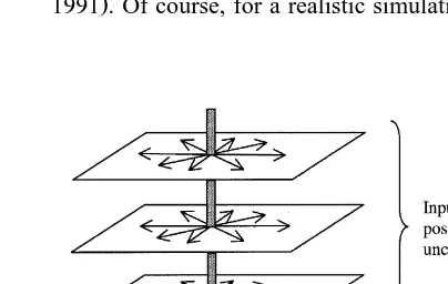
al. 1991 . A typical path taken by data captured by satellite, then abstracted into a suitable form for GIS is shown in Fig. 1, and involves four such models. Continuously varying fields are quantised by the sensing device into image form, then classified and finally transformed into discrete mapping objects. The overall object extraction process is sometimes
Ž
referred to as semantic abstraction Waterfeld and .
Schek, 1992 due to the increasing semantic content of the data as it is manipulated into forms that are easier for people to work with.
1.2. Problem definition
[image:2.595.290.499.563.600.2]When transforming data between different con-ceptual models of geographic space, the uncertainty
characteristics in the data may change; in that tech-niques used to transform the data also alter the inherent uncertainty and in addition may introduce further uncertainty of their own. Furthermore, many of the abstraction techniques employed combine data with different uncertainty characteristics, for
exam-Ž
ple multi-temporal image classification Jeon and
.
Landgrebe, 1992 or knowledge-based feature
extrac-Ž .
tion McKeown, 1987 . Consequently, two inter-re-lated problems must be addressed, namely:
1. How do the uncertainty characteristics of data change as data are transformed between models? 2. How do the transformation methods used affect and combine the uncertainty present in the data ŽLodwick et al., 1990 ?.
This paper concentrates mainly on the first question, proposing a framework within which the second question can be tackled.
One of the consequences of the separation of GIS and RS activities into separate communities and separate software environments is that there is an artificial barrier between the two disciplines. Thus, the integration of these two branches of science is to some extent an artificial problem. As a result, there is no easy flow of meta-data between systems, inter-operability is often restricted to the exchange of image files or object geometry and the problem of managing uncertainty is compounded.
The four stages shown in Fig. 1 represent four models of geographic space that are considered here.
Ž . Ž . Ž .
They are termed the field F , image I , thematic T
Ž . Ž .
and object or feature O models and are typical
Žthough not exhaustive of those used in the integra-.
tion of GIS and remote sensing activities. These models represent the conceptual properties of the data only and are considered here as independent from any particular data structure that might be used to encode and organise the data.
The description of uncertainty used here follows
Ž .
that proposed by Sinton 1978 . It covers the sources of error as they occur in remote sensing and GIS
Ž
integration although other approaches may be
.
equally valid . Uncertainty is restricted to the
follow-Ž . Ž
ing properties: i value including measurement and
. Ž . Ž . Ž .
label errors , ii spatial, iii temporal, iv
consis-Ž .
tency and v completeness. These are symbolised below using the following five letters of the Greek
Ž .
alphabet a, b, x, d and ´, respectively . Of these,
a, b and x can be applied either individually to a
single datum or to any set of data. The latter two properties of consistency and completeness can only apply to a defined data set since they are
compara-Ž
tive either internally among data or to some external .
framework . Issues regarding scale and resolution of
Ž .
the data e.g. Bruegger, 1995 are postponed; these are not objective uncertainty criteria, but instead become important when assessing the ‘fitness for use’ of data for a specific task. Also, we do not concern ourselves here with structures for the
provi-Ž .
sion of lineage information e.g. Lanter, 1991 , al-though these are certainly required to support the propagation of uncertainty.
The techniques proposed for quantifying error and uncertainty referred to in this paper are not in them-selves new. The purpose of the formal notation developed later is to describe succinctly and unam-biguously the forms of uncertainty that exist in the data, where they originate from and what they affect. Ongoing work by the authors and others is attempt-ing to quantify some of these uncertainty terms as they relate to the integration of GIS and remote sensing, for example ISPRS Commissions 2, 3 and 4 span the full range of integration activities described
Ž
here see: http:rrwww.isprs.orgrtechnical com-–
. missions.html for more details .
2. Description of data model properties and their uncertainty characteristics
Ž . More formally, a single geographic datum a at any level of abstraction can be described by its value Ž .d , spatial extents Ž .s and temporal extents Ž .t
ŽGahegan, 1996 each of which have associated un-.
certainty u; where u has three components, a, b
and x
a d, s,t ,
Ž
a,b,x.
.Ž .
1The above expression assumes that a, b and x
formula-tion, using upper case letters, describes a data set, Ž .
but now also includes terms for consistency d and
Ž .
completeness ´
A D,S,T ,
Ž
a,b,x,d,´.
.Ž .
2Each datum exists only within the geographic model under which it was captured or made, so a description of a datum or data set includes a
refer-ence to a conceptual model, C , as shown above,x
where COsobject, CTsthematic, CIsimage and
CFsfield
A D,S,T ,
Ž
a,b,x,d,´. Ž
: Cx.
.Ž .
3The transformations shown in Fig. 1 may be described generally by
A C
Ž
F.
™AXŽ
CI.
™AYŽ
CT.
™AXYŽ
CO.
Ž .
4where each transformation modifies the data charac-teristics described above. At each stage in the pro-cess, a new data set is created, having modified values for some or all of the above properties. The following section describes these properties as they apply to the four conceptual models considered here. Following from this, the outcome of the transforma-tion process on these properties is described, provid-ing one way to specify the effects of these transfor-mations on all the properties of a data set given above.
Ž .
Veregin 1989 defines two distinct categories of Ž .
uncertainty as: i ‘error propagation’, describing the manner in which error accumulates during
process-Ž .
ing and ii ‘error production’, defined as the intro-duction of error by the use of incorrect procedures or data. Here we note that ‘error production’ must be widened to include errors induced by the process of semantic abstraction. Each of the transformations shown in Fig. 1 have a quantising or generalising effect on the data, changing the nature of the data value and its inherent uncertainty. Specifically, these include gridding error, classification error, object recognition and object definition error.
As described in Section 1, the aim of this research is to account for all the types of uncertainty that are present or have risen in data sets as they undergo processing and transformation. Since uncertainty does not just ‘happen’, each uncertain term must originate from some data source or process, and thus may be
accounted for. Therefore, if an uncertainty term ap-Ž pears on the right hand side of any expression Eq.
.
5 , then a corresponding term must occur within at
Ž . Ž. Ž
least one of: i the input data sets A left hand
. Ž .
side , ii as a consequence of the transformationC
Ž . Ž .
or iii as additional data Q used by a transforma-Ž
tion such as spectral training pixels or ground
con-Ž ..
trol points GCPs
C X
A
Ž .
™ A .Ž .
Ž .
5Q
The origins of each uncertainty term are thus described in a straightforward manner, to which simple rules may be applied to advise of potential mistakes, inconsistencies and invalid assumptions. Section 3 attempts to describe these sources of un-certainty, where they originate from and what effect they have.
3. The transformation process between geo-graphic models
This section describes the three transformation
processes between geographic models, field™
image, image™theme and theme™object and their
effects on the data characteristics introduced above.
(
3.1. From field model to image model image cap-)
ture
Remote sensing devices sample the physical fields produced by different forms of electro-magnetic ra-diation from which an image ‘snapshot’ is captured. Hence, the act of image capture is actually a trans-formation from the field model to the image model.
A D,S,T : C
Ž
. Ž
F.
™AXŽ
DX,SX,T ,a,b,d. Ž
: C .I.
6
Ž .
The above expression implies the following.
Ž .1 The objective reality of the sensed radiation is
assumed to contain no errors, so the left side of the expression has no uncertainty terms.
Ž .2 A change in the set of data values, D, occurs
sensor design and operation. Consequently, the right Ž
side gains a term for value uncertainty, a.
Incon-sistent response across the sensor due to manufactur-ing or operatmanufactur-ing discrepancy and sensor drift may
also add to a, but an attempt is usually made to
. remove these effects by a calibration correction .
Ž .3 A change in S is enforced by the gridding
process, i.e. spatial quantisation, and is also subject to sensor design and operation. Spatial uncertainty
Žb. is introduced as a result of gridding since the
geometry of the sensing process usually produces pixels which represent different sized regions, due to the combination of platform position and attitude, sensing angle and landscape topography. That
por-tion of b due to the sensor can be described by a
function applied across all pixels, according to their position, so that it is consistent. Distortion due to relief is inconsistent and can be significant in moun-tainous or built up areas and requires an elevation model for correction.
Ž .4 No term for temporal uncertainty is required.
In most practical cases, image capture may be
as-Ž .
sumed to be instantaneous denoted by T and known within the accuracy required for analysis. A single instantaneous value is, therefore, sufficient. How-ever, there are examples where the sensing cycle is not negligible, such as when a mosaic scene is being produced from collections of aerial photographs.
Ž .5 The image is assumed to be complete but not
necessarily consistent, hence the introduction of d in
the result. Completeness is achieved since each pixel has a value, and consistency may be achieved if all pixels are sensed in the same manner. In practice, the image may not be gathered consistently due to par-tial cloud or some other atmospheric condition
ŽKaufman, 1988 . For example, the reflected signal.
is effectively filtered by the intervening space. The filter itself is inconsistent and may vary spatially, hence the introduction of the uncertainty term for value and consistency. For satellites such as Landsat TM, it is not possible to be certain of the extent of atmospheric effects since no part of the sensor can quantify their presence. However, it is a usual prac-tice to try to work with images that appear to be consistent and the processing techniques that are applied often assume image consistency.
After being captured, the image data often under-goes a number of additional processes in order to
prepare it for further analysis. Each of these transfor-mations may be described with a similar expression to that given above, except that they all retain the image as a basis so no model transformation occurs. Three common examples follow.
Registration, by the use of GCPs, introduces an additional form of spatial uncertainty due to the positional error in the GCPs themselves and the algorithm used to perform the image resampling. The nearest neighbour resampling method does not
Ž .
change pixel values D but does affect the
uncer-Ž .
tainty of these values a due to translation
A D,S,T ,
Ž
a,b,d.
Cregistration
X X X X
6 A D,S ,T ,
Ž
a ,b ,d,´.
.Ž .
7Ž .
GCPs S ,b,´
Interpolation using bilinear or cubic methods ad-ditionally modifies data values as well as adding to Ž . value uncertainty, by changing the spatial basis S and then re-apportioning the data to it
A D,S,T ,
Ž
a,b,d,´.
Cresampling
X X X X X
6 A D ,S ,T ,
Ž
a ,b ,d,´.
.Ž .
8 XŽ .
Grid S
Ž
Certain image enhancement methods such as
.
contrast stretching may also dramatically change the data values, although they usually preserve the order-ing of any trends.
A D,S,T ,
Ž
a,b,d,´.
Ccontrast stretch– 6 A D ,S,T ,X X X
a ,b,d,´ . 9
Ž
.
Ž .
The above expressions show that apart from un-certainty inherent in the image acquisition process itself, associated pre-processing activities introduce a variety of data and spatial uncertainty that accumu-lates at each successive transformation.
( 3.2. From image model to thematic model image
) classification
Ž .
terms by replacing a multi-valued sensor reading Ž
with a single class label i.e. the value element in the .
data description changes type . Measurement errors no longer apply but are replaced with measures of confidence in the labelling process. It is common to use some form of supervised classification as the transformation process, in which case each theme or class is described in terms of examples or average characteristics.
Individual image pixels will have a different re-Ž
sponse to the classifier for a maximum likelihood
Ž .
classifier MLC this can be quantified in terms of .
posterior probability values . So, the thematic value error applies on a per-pixel basis, but may be sum-marised by class for the entire coverage. If we regard the classification process simply in terms of chang-ing the value associated with a pixel, then we may
divorce a and b, since we need never be concerned
as to the overall shape of a class or theme. However, this does not help the user who wishes to understand the likely accuracy of a boundary, or the chances that an object is incorrectly segmented or labelled. This issue is thus carried over from the thematic model into the object model and is described in Section 3.3. Many different approaches to classification are possible, employing a wide range of additional data sources. Some distinct scenarios are considered be-low.
3.2.1. Single image classification Ž .
For each pixel, the image data D are replaced Ž X
.
with class labels D . The expression shown below is of a MLC, an example of a supervised classifier. Supervised classification uses data examples for
Ž .
training from which k class descriptions Q1 . . . k are
created as probability density functions. These de-scriptions act as a controlling input to the
classifica-Ž .
tion processC but are not changed by it , and are
shown under the transformation arrow.
The spatial extents of the class descriptions used Ž ).
for training, Q S are assumed to be the entire
) Ž .
coverage; S is given by the spatial extents of A S .
In other words, we assume the class descriptions can be applied to any pixel in the image. It is interesting to note that each class description has, in theory at least, completeness and consistency properties that describe the validity of this assumption. Since the
class descriptions are used comparatively for la-belling, any uncertainty they possess is likely to
X Ž .
increase the final labelling uncertainty, A a
A D,S,T ,
Ž
a,b,d. Ž
: CI.
CMLC 6
)
Q1ŽD , S ,T ,1 a1,d ´1 1.
)
Q2ŽD , S ,T ,2 a2,d2,´2.. . .
5
)
QkŽD , S ,T ,k ak,dk,´k. AX DX,S,T ,aX
,b,dX
,´ : C . 10
Ž
. Ž
T.
Ž
.
The following points also apply.
Ž .1 D properties change from a vector of
quantita-Ž
tive values to a single class label or possibly a . probabilistic label vector if the classification is ‘soft’ .
Ž .2 S and b properties remain unchanged. The
spatial basis of the image is retained, so S and b are
not affected.
Ž .3 T properties remain unchanged; the resulting
classes represent an interpretation of a single image in isolation so no temporal uncertainty is introduced by the classification process. This and the previous
Ž . Ž . Ž .
point assume that A S sQ S1 . . . k and A T s
Ž .
Q T1 . . . k , i.e. the training values are drawn from A.
Ž . Ž .
Major problems may occur if A S /Q S1 . . . k or
Ž . Ž .
A T sQ T1 . . . k , since the training data are repre-sentatives of different place or time, giving rise to
Ž .
spatial or temporal inconsistency Section 3.2.3 .
Ž .4 a must either expand or change to include the
uncertainty in the class labelling process, on a per-pixel basis, to represent our confidence in the classi-fier.
Ž .5 Completeness may be an issue since the
de-fined classes themselves may not cover all possibili-ties. Pixels may be left unassigned or lumped to-gether into an ‘unknown’ class; the partitioning of pixels into classes is thus incomplete. Any such problems originate with the training data in terms of how well each individual class is described. This is shown by the value and completeness uncertainty terms in the description of Q1 . . . k, and is carried over
into the result, AX. In the case of completeness, a
new error term is introduced into the result as a
consequence. Of course, these uncertainties in AX are
represent the consequences of uncertainty in A and Q as manifested in the thematic model.
Ž .6 It is normal for a consistent approach to
classification to be taken, where all pixels are treated exactly the same by the classifying algorithm; that being the case, no further consistency error is
intro-duced byCML C.
The accumulation of uncertainty from one model to another is certainly not straightforward; large but consistent ‘errors’ in recorded pixel reflectance val-ues may have little influence on classification accu-racy. For example, reflectance values in Landsat TM may be attenuated by up to 40% by non-obvious
Ž Ž . .
atmospheric effects i.e. A a s40% . However,
this results only in a reduction of the dynamic range of the data; the ability of a classifier to separate out the themes will be impaired by a much smaller amount — provided, of course, that the training data values are taken from the affected image. Inconsis-tencies in the attenuation are likely to have a much greater effect than the attenuation itself. Another related problem may arise from effects introduced by terrain variations, e.g. shadows within otherwise consistent classes that cause misclassifications.
3.2.2. Multi-temporal image classification
Now we consider the case where the same sensor provides two or more temporally separated images
Ž that are used together as input to the classifier Jeon
.
and Landgrebe, 1992 , shown by
A1
Ž
D ,S,T ,1 1 a1,b1,d1. Ž
: CI.
•
A2
Ž
D ,S,T ,2 2 a2,b2,d2. Ž
: CI.
. . .ß
An
Ž
D ,S,T ,n n an,bn,dn. Ž
: CI.
CMLC 6
)
Q1ŽD , S ,T ,1 a1,d ´1 1.
)
Q2ŽD , S ,T ,2 a2,d2,´2.. . .
5
)
QkŽD , S ,T ,k ak,dk,´k. AX DX,S,TX,aX
,bX ,dX
,´ : C . 11
Ž
. Ž
T.
Ž
.
It is assumed that all images are co-registered and Ž .
therefore share the same spatial basis S with known uncertaintyb1 . . . n. As before, temporal uncertainty is not an issue, since the capture date and time for each image should be known accurately. However, the
time represented by the resulting classified overlay poses a philosophical problem. The contributing im-ages each represent different dates, possibly from
Ž
different seasons perhaps to improve crop
differenti-. Ž
ation or from different years but the same season to .
study landcover change . In either case, the input data represents several discrete points in time, be-tween which we know nothing but may infer much due to knowledge of plant growth, cropping patterns and so forth. In the former case, we are inferring a continuation in landcover type, using evidence from several epochs to differentiate between classes that may be largely inseparable using only a single scene. In the latter case, the classes created represent types of change, rather than types of landcover. So, in both cases the resulting temporal property should
repre-Ž .
sent the convex temporal interval covering all
ob-Ž .
served times, as described by Ladkin 1986 . That being the case, the resulting temporal interval is given by first calculating the union of all contribut-ing times and then formcontribut-ing the interval that exactly
spans the resulting set T) as
n
)
TsConvex Interval T
ž
sD
T .i/
Ž
12.
is1
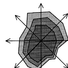
As Fig. 2 shows, each of the input data sets can legitimately take any location within a positional
Ž .
uncertainty band Shi, 1994 , and each possible com-bination of locations produces an equally viable the-matic coverage. Such perturbations can be simulated
Ž
using Monte Carlo techniques e.g. Openshaw et al., .
[image:7.595.293.495.470.598.2]1991 . Of course, for a realistic simulation, the other
Ž
forms of uncertainty such as value error and grid .
distortion must also be varied concurrently.
In the absence of any bias, the results of any such simulation will show central tendency since the error measures represent distributions where values at the extremes are rarer. Consequently, the straightforward combination of the data, ignoring the uncertainty, is likely to produce the best estimate. However, knowl-edge of the uncertainty can be useful in ascertaining the reliability of this result. From the perspective of classification, what is most interesting is not the uncertainty envelopes per se, but rather where the conjunction of uncertainty measures can give rise to a different interpretation — i.e. a different class label assigned to a pixel. A practical goal is therefore to be able to report, for each pixel, whether there is scope within the accumulated uncertainty for a dif-ferent outcome to have occurred, and its likelihood.
3.2.3. Single image classification using ancillary data sources
Two scenarios are considered. In the first, an Ž
existing spatial framework is provided for example, . a set of field boundaries from a GIS coverage to
Ž
which labels are to be added for example, the crop .
type . The spatial framework in data set A imposes2
Ž .
geometric constraints object shapes onto the classi-fier. As before, the labelling, uncertainty originates
Ž .
entirely from the image data D1 but now the
Ž .
spatial uncertainty b of the result is determined by
Ž .
the boundary data set S2 and by the positional error
Ž .
of the image S :1
A1
Ž
D ,S ,T ,1 1 1 a1,b1,d1. Ž
: CI.
5
A2Ž
D ,S ,T ,2 2 2 a2,b2,x2,d2,´2. Ž
: CO.
CLABELLING 6
)
Q1ŽD , S ,T ,1 a1,d1,´1.
)
Q2ŽD , S ,T ,2 a2,d2,´2.. . .
5
)
QkŽD , S ,T ,k ak,dk,´k.
AR
Ž
D ,S ,T ,R R R aR,bR,xR,dR,´R. Ž
: CO.
.Ž
13.
Notice that this expression contains a mix of concep-tual models. The labelling method must resolve this
difference somehow before the image and object data may be successfully merged.
The second scenario is so-called ‘contextual’
clas-Ž .
sification as described by Gurney 1983 , where
Ž
many different ancillary data layers such as soil .
type and elevation are added into the process with the aim of improving class differentiation
A1
Ž
D ,S,T ,1 1 a1,b,d1. Ž
: CI.
•
A2
Ž
D ,S,T ,2 2 a2,b2,x2,d2,´2. Ž
: CI.
. . .ß
An
Ž
D ,S,T ,n n an,bn,xn,dn,´n. Ž
: CI.
CMLC 6
)
Q1ŽD , S ,T ,1 a1,d1,´1.
)
Q2ŽD , S ,T ,2 a2,d2,´2.. . .
5
)
QkŽD , S ,T ,k ak,dk,´k.
AR
Ž
D ,S ,T ,R R R aR,bR,xR,dR,´R. Ž
: CT.
.Ž
14.
In addition to the uncertainty described in the previous example, further uncertainties may arise as a result of the possible mismatch between the S and T properties of all input data sets A1 . . . n. These data sets must each provide data values for a set of given spatial locations, defined by each pixel in the image,
i.e., the value of d and a must be determined in A ,2
. . . , A for each pixel location in all input data sets;n a task which may require registration if these data sets do not share the same spatial structure as the
Ž .
image. As previously described Section 3.1 , regis-tration carries its own data uncertainty legacy.
Ž .
For a given pixel or spatial location s , the class label produced is typically a function of the data
Ž .
values in each data set Heuvelink et al., 1989
AX
Ž
dX, s.
sf A d , s , AŽ
1Ž
1.
2Ž
d , s , . . . A2.
nŽ
d , sn.
.
, 15Ž
.
where f might represent a MLC. In a similar
man-ner, the resulting uncertainty term in a represents
Ž .
some usually unknown function applied across the value uncertainty of each contributing layer at the same location, described as
AX s,aX
sf A s,a , A s,a , . . . A s,a .
Ž
.
Ž
1Ž
1.
2Ž
2.
nŽ
n.
.
16
However, in practice a is defined not by the input data uncertainty, but by the posterior probabilities of the classification process, and most commonly by the sum of the posterior probabilities excluding the
dom-Ž . inant class q , i.e.
k
X X X X
A s,
Ž
a.
sÝ
P A d , sŽ
Ž
.
si.
i/q.Ž
17.
is1
The above expression ignores the uncertainty already present in the image data, which in turn may lead to an overestimate of the reliability of the result.
Temporal uncertainty may arise when data is used to represent a time other than that at which it was gathered. This does not apply to the previous cases
Ždescribed in Section 3.2.2 , since the data is used.
according to the time it was captured. However, where different ancillary data sets are included, then temporal uncertainty may creep in. Examples include the use of historically averaged rainfall data, the assumption being that the same values apply over an instantaneous image, or where data from previous
Ž .
times e.g. years are used by necessity. The ‘tem-poral distance’ between two data sets is difficult to quantify and depends on the nature of the data concerned and the rate at which it changes. For example, a geology map is unlikely to become out of date within the lifetime of a system, but a remotely sensed image might become obsolete in a matter of days. Such data is cyclic in its usefulness, but not perfectly so, since two images 1 year apart will not represent the same point in the season — the envi-ronmental conditions may well be different.
3.2.4. Multi-sensor classification
Where images are acquired from different
plat-Ž .
forms and combined fused in the classification
process, then the data will initially exist in two
different spatial bases, hence S1/S . The resulting2
grid is usually that of the data set with the highest
Ž .
resolution, so SRsmax resolution S , S . Spatial1 2
uncertainty becomes dependent on both b1 and b2.
Ž .
As in the collaborative labelling example Eq. 13 above, the method employed must be more sophisti-cated than a conventional classifier, to manage the conflicting spatial bases.
A1
Ž
D ,S ,T ,1 1 1 a1,b1,d1. Ž
: CI.
5
A2Ž
D ,S ,T ,2 2 2 a2,b2,d2. Ž
: CI.
CFUSION 6
)
Q1ŽD , S ,T ,1 a1,d1,´1.
)
Q2ŽD , S ,T ,2 a2,d2,´2.. . .
5
)
QkŽD , S ,T ,k ak,dk,´k.
AR
Ž
D ,S ,T ,R R R aR,bR,xR,dR,´R. Ž
: CT.
.Ž
18.
3.3. From thematic model to object model
An object is considered here as an independent entity with a defined shape; any pixels incorrectly included or excluded from the entity will cause the shape to be in error. This gives rise to a new dimension of spatial uncertainty in the object model
Ž due to the need to define the shape property unlike a
.
pixel, whose shape is given . The object model thus has shape error, which is treated here as an extension
of b into the object model. Any positional error
inherited from the image data remains, and becomes positional error in objects derived from this data. It is typical in remote sensing applications that classifica-tion errors tend to occur around the edges of objects
ŽShi, 1994 , due to transition zones and mixed pixel.
effects. It is also typical of some types of objects that they do not possess discrete boundaries to begin with
ŽBurrough, 1989; Edwards and Lowell, 1996 . Fig. 3.
shows two different types of spatial error for a given area object. The arrows represent positional error, while the different shadings represent possible shapes for the object.
In a similar manner, a must expand to include
identity uncertainty, representing the chances that the object is incorrectly ‘typed’, perhaps as a result of classification uncertainty
A D,S,T ,
Ž
a,b,x,d,´. Ž
: CT.
CObject Formation
6
Object Formation Rules
AX DX,SX,T ,aX ,bX
,x,dX ,´X
: C . 19
Fig. 3. Two forms of spatial uncertainty in an object, inherited from the image from which it was formed and due to uncertainty in boundary delineation and position.
Ž .
Gahegan and Flack 1999 provide one possible ap-proach to combine attribute and positional uncer-tainty encountered during object formation using
Ž
Dempster–Shafer evidential reasoning Shafer,
. 1976 .
Another source of uncertainty within the object model is that of defining the objects themselves. These are typically imprecise, if defined in terms of image properties, or difficult to quantify, if defined in high-level terms such as those suggested by Kuhn
Ž1994 . Consequently, object types which are impre-. Ž
.
cise pass on uncertainty to object instantiations as an additional facet to object identity uncertainty
de-scribed bya.
Most object formation strategies function basi-cally the same way, although they differ in complex-ity of reasoning — an object acquires its label due to passing a threshold of similar or identically labelled pixels within a hypothesised region. Where uncer-tainty is high, it is possible that a predominance of different values or labels might arise under different instantiations of the uncertainty components, leading to a different object being formed.
Ž . This situation is most likely to occur where: i
Ž .
the object itself is small, ii positional error is large Ž .
and iii the values or class labels are ‘close’ or Ž
overlap in other words, differentiation is poor or the .
classification scheme is inappropriate . Reporting methods exist in remote sensing to identify this latter problem, such as the classifier accuracy table show-ing errors of omission and commission, but there is no counterpart in the object domain.
3.3.1. From image model directly to object model Some object extraction strategies bypass the clas-sification stage altogether. These strategies differ greatly in terms of their complexity, their data re-quirements and their organisation. At one extreme, objects may be formed by directly interpreting the image data manually, as with ‘heads up’ digitising from an image on the display screen. At the other extreme, extraction strategies may employ sophisti-cated pattern recognition tools and high-level
reason-Ž
ing McKeown, 1987; Matsuyama and Hwang, 1990; .
Gahegan and Flack, 1996; 1999 . Such strategies make use of a variety of transformations that are not covered here. A useful overview of the general approach to object recognition taken in computer
Ž .
vision is given by Sonka et al. 1993, p. 43 .
4. Discussion, conclusions and future work
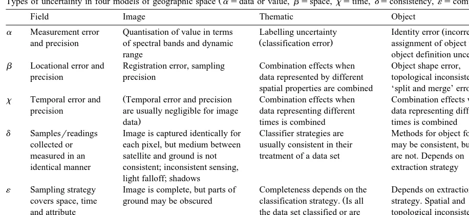
The expressions described above seem to offer some insight into the complex transformation pro-cesses that occur within integrated GIS, particularly with reference to keeping track of the sources of errors and uncertainties and their effects. Table 1 categorises these errors and uncertainties as they apply to the four geographic models considered here. Uncertainty propagates from left to right across the table as the higher models inherit uncertainty properties from the lower models and add to this their own specific measures. Of course, the increase in uncertainty is accompanied by a corresponding information ‘gain’ as a result of semantic abstraction — the identity of the data becomes more certain as the associated properties become less certain. For example, a thematic map may inherit data uncer-tainty from the imaging process as well as acquiring further label uncertainty through the imperfections of the classification process, but the result is a higher
semantic entity. So, for example a value taken by a
for a thematic data set must account for the data Ž .
error in the input data set s as well as the classifier labelling uncertainty, L
Table 1
Ž .
Types of uncertainty in four models of geographic space asdata or value,bsspace,xstime,dsconsistency,´scompleteness
Field Image Thematic Object
Ž
a Measurement error Quantisation of value in terms Labelling uncertainty Identity error incorrect
Ž . .
and precision of spectral bands and dynamic classification error assignment of object type ,
range object definition uncertainty
b Locational error and Registration error, sampling Combination effects when Object shape error,
precision precision data represented by different topological inconsistency,
spatial properties are combined ‘split and merge’ errors
Ž
x Temporal error and Temporal error and precision Combination effects when Combination effects when precision are usually negligible for image data representing different data representing different
.
data times is combined times is combined
d Samplesrreadings Image is captured identically for Classifier strategies are Methods for object formation collected or each pixel, but medium between usually consistent in their may be consistent, but often measured in an satellite and ground is not treatment of a data set are not. Depends on
identical manner consistent; inconsistent sensing, extraction strategy
light falloff; shadows
´ Sampling strategy Image is complete, but parts of Completeness depends on the Depends on extraction
Ž
covers space, time ground may be obscured classification strategy. Is all strategy. Spatial and
and attribute the data set classified or are topological inconsistencies
.
domains adequately only some classes extracted? may arise as a result of object formation
The definition of the combination operator, [, is
Ž .
itself problematic. As Veregin 1989 shows, it is rarely appropriate to simply add the uncertainty terms together.
As semantic abstraction progresses, the ‘fitness for use’ of the data also changes; it becomes more readily used as an identifiable object as opposed to a continuous field. A question remains as to whether
Ž .
the associated loss of data i.e. variance should
cause an uncertainty penalisation. We can be certain of the identity of the model to which the datum belongs, so there should be no mistakes in interpret-ing what the value represents. Therefore, abstraction should not necessarily, in itself, incur an uncertainty penalty. Classes are defined as collections with
vari-Ž .
ance e.g. MLC so they already represent variance in a summarised form. However, definitions for ob-jects in terms of variance and uncertainty are yet to be fully developed and represent a real barrier to progress at present. Quantifying the performance of object formation has become a lively area of debate
Ž
among the computer vision community e.g. Haral-.
ick, 1994 , but a good deal more research is required before this final stage of model transformation can be fully understood and effectively communicated.
Perhaps the most difficult aspect of managing uncertainty in an integrated GIS is the inter-relation-ship between the various types of uncertainty
de-scribed. For example, a and b strongly influence
each other; an incorrect data value for a pixel may ultimately result in an object being assigned the ‘wrong’ shape. Conversely, positional errors in im-age data may lead to mis-classification. In data
modelling terms, we say that a and b are
function-ally dependent on each other
a´bandb´a.
Ž
21.
Such circular referencing is not easily resolvable, but occurs as a consequence of moving from one model of space to another. Simulation and experimentation offer a way of understanding these inter-relation-ships, but new forms of metrics will be required to describe them.
Consistency and completeness are extremely problematic to describe, since they relate to the nature of variance of error over a coverage, and are
thus a summary of the effects of a, b and x. In
many cases, acceptable metrics for d and ´ are
defined. Furthermore, their combination through transformation has not been addressed, as yet.
The approach described in this paper is currently being used as the basis for a simulation package, developed in an attempt to model these various forms of uncertainty in order to test their inter-rela-tionships and to evolve better ways of assessing and reporting their significance.
References
Bedard, Y., 1987. Uncertainties in land information databases. Proc. Auto-Carto 8, Baltimore, pp. 175–184.
Bruegger, B.P., 1995. Theory for the integration of scale and representation formats: major concepts and practical
implica-Ž .
tions. In: Frank, A.U., Kuhn, W. Eds. , Spatial Information Theory, Lecture Notes in Computer Science vol. 988 Springer Verlag, Berlin, pp. 297–310.
Burrough, P.A., 1989. Fuzzy mathematical methods for soil
sur-Ž .
vey and land evaluation. J. Soil Sci. 40 3 , 477–492. Chrisman, N.R., 1991. The error component in spatial data. In:
Ž .
Maguire, D.J., Goodchild, M.F., Rhind, D.W. Eds. , Geo-graphical Information Systems vol. 1 Longman, pp. 165–174, Principles.
Edwards, G., Lowell, K.E., 1996. Modelling uncertainty in photo-interpreted boundaries. Photogramm. Eng. Remote Sens.
Ž .
62 4 , 377–391.
Ehlers, M., Greenlee, D., Smith, T., Star, J., 1991. Integration of remote sensing and GIS: data and data access. Photogramm.
Ž .
Eng. Remote Sens. 57 6 , 669–675.
Ehlers, M., Shi, W., 1997. Error modelling for integrated GIS.
Ž .
Cartographica 33 1 , 11–21.
Gahegan, M.N., 1996. Specifying the transformations within and
Ž .
between geographic data models. Trans. GIS 1 2 , 137–152. Gahegan, M.N., Flack, J.C., 1996. A model to support the integra-tion of image understanding techniques within a GIS.
Pho-Ž .
togramm. Eng. Remote Sens. 62 5 , 483–490.
Gahegan, M., Flack, J.C., 1999. Recent developments towards integrating scene understanding within a geographic
informa-Ž .
tion system for agricultural applications. Trans. GIS 3 1 , 31–50.
Ž .
Goodchild, M.F., Gopal, S. Eds. , The Accuracy of Spatial Databases. Taylor & Francis, London.
Goodchild, M.F., 1992. Geographical data modelling. Comput.
Ž .
Geosci. 18 4 , 401–408.
Goodchild, M.F., Guoqing, S., Shiren, Y., 1992. Development and test of an error model for categorical data. Int. J. Geogr. Inf.
Ž .
Syst. 6 2 , 87–104.
Gurney, C.M., 1983. The use of contextual information in the classification of remotely sensed data. Photogramm. Eng.
Re-Ž .
mote Sens. 49 1 , 55–64.
Haralick, R.M., 1994. Performance characterisation in computer
Ž .
vision. CVGIP-Image Understanding 60 2 , 245–249.
Heuvelink, G.B.M., Burrough, P.A., Stein, A., 1989. Propagation of errors in spatial modelling with GIS. Int. J. Geogr. Inf. Syst.
Ž .
3 4 , 303–322.
Heuvelink, G.B.M., Burrough, P.A., 1993. Error propagation in cartographic modelling using Boolean logic and continuous
Ž .
classification. Int. J. Geogr. Inf. Syst. 7 3 , 231–246. Hunter, G., Goodchild, M.F., 1993. Mapping uncertainty in spatial
databases, putting theory into practice. J. Urban Reg. Inf. Syst.
Ž .
Assoc. 5 2 , 55–62.
Hunter, G., Goodchild, M.F., 1996. Communicating uncertainty in
Ž .
spatial databases. Trans. GIS 1 1 , 13–24.
Jeon, B., Landgrebe, D.A., 1992. Classification with spatio-tem-poral interpixel class dependency contexts. IEEE Trans.
Ž .
Geosci. Remote Sens. 30 4 , 663–672.
Kaufman, Y., 1988. Atmospheric effect on spectral signature — measurements and corrections. IEEE Trans. Geosci. Remote
Ž .
Sens. 26 4 , 441–450.
Kuhn, W., 1994. Defining semantics for spatial data transfers. In:
Ž .
Waugh, T.C., Healey, R.G. Eds. , Proc. 6th International Symposium on Spatial Data Handling. University of Edin-burgh, Scotland, pp. 973–987.
Ladkin, P., 1986. Time representation: a taxonomy of interval relations. AAAI-86–5th National Conference on Artificial In-telligence vol. 1 Morgan Kaufmann, Philadelphia PA, USA, pp. 360–366.
Lanter, D.P., 1991. Design of a lineage-based meta-data base for
Ž .
GIS. Cartography Geogr. Inf. Syst. 18 4 , 255–261. Leung, Y., Yan, J., 1998. A locational error model for spatial
Ž .
features. Int. J. Geogr. Inf. Sci. 12 6 , 607–620.
Lodwick, W.A., Monson, W., Svoboda, L., 1990. Attribute error and sensitivity analysis of map operations in geographical information systems: suitability analysis. Int. J. Geogr. Inf.
Ž .
Syst. 4 4 , 413–428.
Lunetta, R.S., Congalton, R.G., Fenstermaker, L.K., Jensen, J.R., McGwire, K.C., Tinney, L.R., 1991. Remote sensing and geographic information system data integration: error sources
Ž .
and research issues. Photogramm. Eng. Remote Sens. 57 6 , 677–687.
Matsuyama, T., Hwang, V.S., 1990. Sigma: A Knowledge-Based Aerial Image Understanding System. Plenum, New York. McKeown, D.M. Jr., 1987. The role of artificial intelligence in the
integration of remotely sensed data with geographic
informa-Ž .
tion systems. IEEE Trans. Geosci. Remote Sens. GE-25 3 , 330–348.
Miller, R., Karimi, H., Feuchtwanger, M., 1989. Uncertainty and its management in geographical information systems. Proc. CISM ’89. Canadian Institute of Surveying and Mapping, Ottawa, Canada, pp. 252–259.
Openshaw, S., Charlton, M., Carver, S., 1991. Error propagation: a Monte Carlo simulation. In: Masser, I., Blakemore, M.
ŽEds. , Handling Geographic Information. Longman, England,.
pp. 78–101.
Ruiz, M.O., 1997. A causal analysis of viewshed error. Trans. GIS
Ž .
2 1 , 85–94.
Shafer, G., 1976. A Mathematical Theory of Evidence. Princeton University Press, Princeton NJ, USA.
the integration of remote sensing and geographic information
Ž .
systems. PhD Thesis, ITC publication number 22 , Enschede, The Netherlands.
Sinton, D., 1978. The inherent structure of information as a constraint to analysis: mapped thematic data as a case study.
Ž .
In: Dutton, G. Ed. , Harvard Papers on Geographic Informa-tion Systems vol. 6 Addison-Wesley, Reading MA, USA. Sonka, M., Hlavac, V., Boyle, R., 1993. Image Processing,
Analy-sis and Machine Vision. Chapman & Hall.
Story, M., Congleton, R.G., 1986. Accuracy assessment: a users
Ž .
perspective. Photogramm. Eng. Remote Sens. 52 3 , 397–399. Veregin, H., 1989. Error modelling for the map overlay operation.
Ž .
In: Goodchild, M.F., Gopal, S. Eds. , Accuracy of Spatial Databases. Taylor and Francis, pp. 3–19.
Veregin, H., 1995. Developing and testing of an error propagation model for GIS overlay operations. Int. J. Geogr. Inf. Syst. 9
Ž .6 , 595–619.
Waterfeld, W., Schek, H.-J., 1992. The DASBDS Geokernel —
Ž .
an extensible database system for GIS. In: Turner, A.K. Ed. , Three-Dimensional Modelling with Geoscientific Information Systems. Kluwer Academic Publishing, Netherlands, pp. 45– 55.
Worboys, M., 1998. Computation with imprecise geospatial data.
Ž .