Full Terms & Conditions of access and use can be found at
http://www.tandfonline.com/action/journalInformation?journalCode=ubes20
Download by: [Universitas Maritim Raja Ali Haji] Date: 12 January 2016, At: 22:58
Journal of Business & Economic Statistics
ISSN: 0735-0015 (Print) 1537-2707 (Online) Journal homepage: http://www.tandfonline.com/loi/ubes20
Determining the Number of Primitive Shocks in
Factor Models
Jushan Bai & Serena Ng
To cite this article: Jushan Bai & Serena Ng (2007) Determining the Number of Primitive
Shocks in Factor Models, Journal of Business & Economic Statistics, 25:1, 52-60, DOI: 10.1198/073500106000000413
To link to this article: http://dx.doi.org/10.1198/073500106000000413
Published online: 01 Jan 2012.
Submit your article to this journal
Article views: 273
View related articles
Determining the Number of Primitive Shocks
in Factor Models
Jushan B
AIDepartment of Economics, New York University, 269 Mercer St., New York, NY 10003, and Department of Economics, Tsinghua University, Beijing, China ([email protected])
Serena N
GDepartment of Economics, University of Michigan, Ann Arbor, MI 48109 ([email protected])
A widely held but untested assumption underlying macroeconomic analysis is that the number of shocks driving economic fluctuations,q, is small. In this article we associateqwith the number of dynamic factors in a large panel of data. We propose a methodology to determineqwithout having to estimate the dynamic factors. We first estimate a VAR inrstatic factors, where the factors are obtained by applying the method of principal components to a large panel of data, then compute the eigenvalues of the residual covariance or correlation matrix. We then test whether their eigenvalues satisfy an asymptotically shrinking bound that reflects sampling error. We apply the procedure to determine the number of primitive shocks in a large number of macroeconomic time series. An important aspect of the present analysis is to make precise the relationship between the dynamic factors and the static factors, which is a result of independent interest.
KEY WORDS: Common shocks; Dynamic factor model; Number of factors; Principal components analysis; Static factor.
1. INTRODUCTION
A common working assumption in macroeconomics is that economic fluctuations are driven by a small number of shocks. It would not be too controversial to suggest that the number of shocks is no larger than four. In fact, it is not easy to find a busi-ness cycle model built from microfoundations with more than four shocks. Macroeconomists have been preoccupied with un-derstanding the transmission and quantifying the importance of three shocks: technology, monetary, and fiscal policy. But what is the exact number of primitive shocks in the data? In this ar-ticle we propose a simple testing procedure to determine this number, which we denote byq. More precisely, the qthat we determine is the rank of the spectral density matrix of the com-mon components in a large panel of data or, equivalently, the number of common factors in a dynamic factor model. We do this without having to estimate a dynamic factor model, how-ever.
Surprisingly, few test exists to formally evaluate what is the exact value ofq. Using a dynamic index model to analyze quar-terly data for 14 series over the sample 1950:1–1970:1, Sargent and Sims (1977) rejected the one- and two-index models in fa-vor of a model with more factors, though they noted that the two index model fits the real variables quite well. In two re-cent articles Forni, Giannone, Lippi, and Reichlin (2003) and Giannone, Reichlin, and Sala (2005) argued that the number of macroeconomic shocks, which they referred to as the stochas-tic dimension of the economy, is two. They estimated common factors from quarterly data on 190 series over the sample period 1970–1996 and arrived at the conclusion of two shocks using a reasonable (albeit informal) judgment that two dynamic factors explain about 60% of the variation in 12 macroeconomic aggre-gates. However, this does not mean that two factors is optimal for the panel of data from which the factors are extracted. Fur-thermore, changing the cutoff point from 60% to 80% would lead to a stochastic dimension twice as large. Because there does not exist a formal test for the number of dynamic factors, their conclusion thatq=2 remains very much an assertion.
The analytical framework used by Forni et al. (2003) and Giannone et al. (2005) is the so-called “dynamic factor” model. Like the static factor model favored by Stock and Watson (2002a), the dynamic factor model also summarizes information in a large panel of data using a small number of factors. The important distinction is that rank of the spectrum ofqdynamic factors is alwaysq. Because ther<∞static fac-tors can be dynamically related, the spectrum of r≥q static factors has reduced rank. We can see that this rank is actuallyq, the number of dynamic factors. Accordingly, we refer toq as the number of primitive shocks.
In Section 2 we motivate the procedures in the context of a canonical VAR, in which the number of underlying shocks is less than the number of variables. We formally develop tests for the number of dynamic factors in Sections 3 and 4, and con-sider simulations and an empirical application in Section 5. We present conclusions in Section 6.
2. THE MINIMAL NUMBER OF PRIMITIVE SHOCKS IN VECTOR AUTOREGRESSION
Consider a vector of observed stationary time series,Ft(r× 1),t=1, . . . ,T. Assume thatFt is a VAR process of orderp such that
A(L)Ft=ut, (1)
whereA(L)=I−A1L− · · · −ApLp. Throughout, we assume that the roots ofA(L)=0all lie outside of the unit circle, and theut’s are iid withEut4+δ<M<∞for someδ >0. We consider the case in whichut is driven by a vector of lower-dimensional shocks. Consideration of such a VAR structure is useful in developing our main analysis, which concerns distin-guishing the dynamic factors from the static factors.
© 2007 American Statistical Association Journal of Business & Economic Statistics January 2007, Vol. 25, No. 1 DOI 10.1198/073500106000000413 52
Bai and Ng: Primitive Shocks in Factor Models 53
Definition 1. We say that the VAR process Ft is driven by a minimal number ofqinnovations if there exists ar×q ma-trix,R, with rankqsuch that
ut=Rǫt, (2)
where ǫt is a q×1 vector of innovations that are mutually
uncorrelated; that is, ǫ =E(ǫtǫ′t) is diagonal. If we define
u=E(utu′t), then, under (2),u=RǫR′has rankq≤r.
Bernanke (1986) used ut as the residuals of an estimated VAR and assumedRto be full rank. The number of primitive shocks thus equals the number of variables in the system. We allow the rank ofRto be less thanr. It is in this sense that we are looking for the minimal number of primitive shocks. The number of primitive shocks inutis simply theqlinearly inde-pendent shocks that spanut.
Suppose thatBis an arbitraryr×rmatrix with rankqand that vt is vector of r×1 shocks. Let ut =Bvt. Then ut can be expressed as ut=Rǫt, where Risr×q andǫt is q×1.
To determineq, we use as starting point that ar×r semiposi-tive definite matrixAof rankqhasqnonzero eigenvalues. Let c1>c2≥ · · · ≥cr≥0 be the ordered eigenvalues (at least one
A different interpretation of our test can be obtained using the spectral decomposition ofA,
A=
r
j=1 cjβjβ′j,
where βj is the eigenvector corresponding to cj. Define the
kth pseudomatrix ofAas
A(k)= It follows that our eigenvalue tests are the square root of the deviations from the null hypothesis, as measured by the matrix norm. This follows from trace(βjβ′j)= βj2=1 by construc-tion, andd02=vec(A)′vec(A)=tr(A′A)= A2.
In the next two sections, the matrixA, the rank of which is to be determined, isu, the covariance matrix of a set of
in-novations. Althoughu andFare not observed, they can be
estimated from the data, denoted by ˆu. Let Dˆ1,k and Dˆ2,k
be constructed from the eigenvalues ofˆu. We show thatDˆ1,k
andDˆ2,kconverge to 0 (k≥q) asymptotically at a rate
depend-ing on the convergence rate ofˆutou.
Before turning to our main analysis, a remark on exist-ing rank tests is in order. Available tests seek to determine the rank of a m×n matrix, say R, when R is consistently estimated from the regression ut =Rǫt +vt. Our focus is
on problems in which vt plays no role, but with unobserv-ableut. Furthermore, rank tests tend to not be asymptotically normal (see Anderson 1951; Gill and Lewbel 1992; Cragg and Donald 1996, 1997; Robin and Smith 2000). Recently, Kleibergen and Paap (2006) and Ratsimalahelo (2003) sug-gested orthogonal rotation of the sample eigenvalues around the origin to restore normality. Doing so, these tests necessi-tate a consistent estimate of var(Rˆ). We want to test the rank of the matrixu. This creates two problems. First, estimating
var(ˆu)entails evaluating a matrix of fourth moments, which
tend to be quite imprecisely estimated unless the sample size is extremely large. Second,uis a variance–covariance matrix
that has onlyr(r+1)/2 unique elements; thus var(u)and its
estimate do not have full rank, an assumption maintained by Kleibergen and Paap (2006). The test of Ratsimalahelo (2003) allows for reduced rank in the variance of apparently matrices that are not symmetric. Our attempts to adopt existing tests have not been successful. This motivates the development of a test using bounds guided by the convergence rate ofDˆ1,kandDˆ2,k.
We begin with the intermediate case whenFtis observed butu
is not.
Proposition 1. Let ˆu = T1Tt=1uˆtuˆ′t, where uˆt are the
residuals from estimation of a VAR inFt, whereFtis observed. Let Dˆ1,k and Dˆ2,k be the estimated D1,k and D2,k using the
with probability tending to 1 as T → ∞. This means that q∈K for large T. But q−1 does not belong to K because
ˆ
D1,k>c>0 and thus is>m/T1/2−δfork<q. This gives the
consistency result. Essentially, the cutoff pointm/T1/2−δis the tolerated error induced by sampling variability from estimation ofu. An analogous argument holds forD2,k. In large samples,
the two tests should arrive at the same conclusion.
Thus far, the VAR processFtis assumed to be observed. In the next two sections, Ft is a vector of unobserved common factors shared by a large number of seriesxit.
3. DYNAMIC VERSUS STATIC FACTOR MODELS
There are two types of factor models in the econometrics lit-erature. Thestaticmodel is written asxit=′iFt+eit,where
i=1, . . . ,N,t=1, . . . ,T. In the language of factor analysis,
eitis referred to as the idiosyncratic error, andiis a vector of
factor loadings for uniti on ther(static) common factors Ft. The termstatic factormodel refers to the static relationship be-tweenxitandFt, butFtitself can be a dynamic process. The
dy-namic factormodel is written asxit=λ′i(L)ft+eit, whereλi(L)
is a vector of dynamic factor loadings of order s. As a mat-ter of notation, the model is a “dynamic factor model” if sis finite, and a “generalized dynamic factor model” ifscan be in-finity. In either case,ft=C(L)ǫt, whereǫtare iid vectors and
xit=λi(L)C(L)ǫt+eit. In this article we consider dynamic
fac-tor models (finites). The dimension offt, which is the same as the dimension ofǫt, is called the number of dynamic factors;
and is denoted byq. Dynamic factor models withsfinite can be written as static factor models withrfinite, but the dimen-sion ofFt is in general different from the dimension offt, be-causeFtincludes the leads and lags offtwithr≥q. In practice, Ftis estimated using an eigenvalue–eigenvector decomposition of the sample covariance matrix of the data, whereas the dy-namic estimates are based on a eigenvalue decomposition of the spectrum smoothed over various frequencies. Recent research has shown that the space spanned by the static and dynamic factors can be consistently estimated whenN andT are both large (see, e.g., Forni, Hallin, Lippi, and Reichlin 2000, 2005; Ding and Hwang 2001; Stock and Watson 2002a; Forni and Lippi 2001; Bai and Ng 2002; Bai 2003).
The ability to consistently estimate the factor space has opened up new horizons for empirical research. Using the fac-tor estimates to summarize information in a data-rich environ-ment has been found to be useful in forecasting exercises and in understanding the conduct of monetary policy (see, e.g., Stock and Watson 2002b; Bernanke and Boivin 2003). Although for forecasting purposes, little is to be gained from a clear distinc-tion between the static factors and the dynamic factors, many economic analyses hinge on the ability to isolate the primitive shocks or, in other words, the number of dynamic factors.
In earlier work (Bai and Ng 2002), we showed that under cer-tain conditions, information criteria with appropriately chosen penalties will consistently estimater, whereris assumed finite. We will ultimately propose a way to determineq fromr esti-mated static factors, where ris assumed finite or, in terms of the parameters of the dynamic model,sis finite. But before we can proceed with such an analysis, we need to precisely state the relationship between the dynamic and static factors, treat-ingFt andft as though they are observed. In the remainder of this section, we show that a dynamic factor model always has a static factor representation in which the dynamics ofFtis char-acterized by a VAR with order depending on the dynamics offt. We will see from the VAR representation that the spectrum of the static factors has rankq.
3.1 Putting the Dynamic Model Into Static Form
Consider the dynamic factor model
xit=λ′i0ft+λ′i1ft−1+ · · · +λ′isft−s+eit
=λ′i(L)ft+eit, (5)
whereftisq-dimensional and
λi(L)=λi1+λi2L+ · · · +λisLs. (6)
Clearly we can rewrite (5) in the static form,
xit=′iFt+eit, (7)
The foregoing is a simple mathematical identity and is true whetherft itself is an AR process or an MA process. The di-mension ofFtis always equal to
r=q(s+1),
whereqis the dimension offt. As mentioned earlier, whereas the relation betweenxit andFt is static,Ft itself can be a
dy-namic process with precise characterization depending on the dynamics offt. We consider two cases, one case in whichftis a finite-order AR process, and the other in whichfthas an MA structure.
Case I. ftis AR(h),his finite. In this case,
(Iq−B1L− · · · −BhLh)ft=ǫt. (9)
Note thatftisq-dimensional, and the number of static factors,r, does not depend onh, the order of the dynamic process govern-ingftin (9). Unlesss=0, the number of static factors is larger than the number of dynamic factors.
We now want to establish thatFt is a VAR with order de-pending onh ands. To see the VAR representation of Ft, we q(κ+1)×qmatrix. In traditional state-space representation,
κ=h. In our present case,κ=max(h,s). Ifs≥h, then
Ft≡F∗
t,
so Ft also has a VAR(1) representation. When s<h,Ft is a subvector ofF∗t. In general, any subvector of a VAR is a vector ARMA process, not necessarily VAR. However, due to the spe-cial structure ofF∗
t, the subvectorFtitself is a VAR. This point
Bai and Ng: Primitive Shocks in Factor Models 55
can be easily made clear through an illustration. Suppose that h=3 ands=1, and consider
This implies thatFtis VAR(2). In fact, we can show that for the general situation,Ftis VAR(p)withp=max(1,h−s). There-fore, the dynamic factor model defined by (5)–(6) whenftis a VAR(h) can be written as a static factor model as
Ft=A1Ft−1+A2Ft−2+ · · · +ApFt−p+ut (11)
Under the invertibility assumption, the MA processftcan be expressed as an VAR(∞)process, which can be approximated by a finite-order VAR. This implies thatFtcan also be approxi-mated by a finite-order VAR as in (11) and (12) (see Berk 1974; Kuersteiner 2004 for theoretical results), particularly when the coefficients of the AR process decay quickly to 0. In general, the lag length should be chosen by a data-dependent method and is an increasing function of T. Although this procedure works well in practice, some theoretical issues are left unex-plored when the VAR order increases withT. Proposition 2 is stated only for VARs of fixed orders, and in effect it does not cover case II. Nevertheless, we note that it is possible to extend the theory to include VAR(∞) processes with rapidly decaying coefficients. In particular, the theory can be extended toFt as vector ARMA processes. For simplicity, this extension is not considered here. Monte Carlo simulations show that the proce-dure works well forftas MA processes.
The point that we highlight is that data generated by the dy-namic model can always be mapped into a static model of the formxit=′iFt+eitby suitably defining aFt that evolves
ac-cording to a VAR with order depending on the dynamics offt. The dimension ofFt is alwaysr=q(s+1)irrespective of the order of the VAR. Given thatA(L)Ft=Rǫt, the spectrum ofF
at frequencyω,
SF(ω)=A(e−iω)−1RSǫ(ω)R′A(eiω)−1,
has rankqifSǫ(ω)has rankqfor all|ω| ≤π. Accordingly, the spectrum of the static factorsSF(ω)will also have qnonzero
eigenvalues. Therefore, we refer to the dynamic factors,q, as the number of primitive shocks.
Although the dynamics of the static factors are in the same form as the observable VAR system in (1) in the sense that both are driven by shocks with dimension less than the dimension of the variables, Proposition 1 cannot be used immediately to determineq. This is becauseFt is not observable, and the con-vergence rate ofˆuis not
√
T. We deal with these issues in the next section.
4. DETERMININGq
Let Sx(ω) be the population spectrum of the N
cross-sectional units. The static model implies that
Sx(ω)=SF(ω)′+Se(ω), −π≤ω≤π.
BecauseSe(ω) has rankN,Sx(ω)is also rankN. This would
seem to suggest thatqcannot be determined without working onSF(ω). Such a procedure would necessitate choosing many
auxiliary parameters (such as bandwidth and kernel), and even then, we do not have a formal theory for determiningq. We now show howqcan be estimated in the time domain, with limiting distributions of the eigenvalues unnecessary.
IfFt is observed, and because it has a VAR representation, Proposition 1 then implies that q can be determined from a spectral decomposition of ˆu provided that T is large. What
prevents such an analysis is that neitherFtnor its dimension (r) is observed. However, the following holds. LetFˆr
t be ther
fac-tors obtained by the method of principal components; that is, letˆ be aN×rmatrix consisting of thereigenvectors (mul-tiplied by √N) associated with the r largest eigenvalues of the matrix X′X in decreasing order. ThenFˆ =Xˆ/N. These principal component estimates adopt the normalization that
ˆ
′ˆ/N=Ir. Then, under the assumption that (a)F=E(FtF′t)
and ′/N are both rank r, (b) moment restrictions are sat-isfied, and (c) the time and cross-sectional correlation in the idiosyncratic errors is weak, Bai and Ng (2002) and Bai (2003) showed that if the data are generated by the static factor model, then asN,T→ ∞, there exists a matrixHof rankr, such that
Importantly, the foregoing large-sample results assume that the second moment matrix ofiandFtis rankr. ButFmay
have rank less than r. For example, if Ft =AFt−1+Rǫt is
such that A=ρIr,|ρ|<1, then var(Ft)=RǫR′/(1−ρ2),
var(Ft)has only rankr∗=q. In general, when the dynamics of Ft is sufficiently rich, var(Ft)is of rank reven though the rank of u is onlyq. But existing results do not cover cases
when var(Ft) <r, which can arise as in the foregoing example whenFthas very simple dynamics. We now extend our results on determining the number of factors to also cover these special cases. factor estimates obtained by the method of principle com-ponents. There exists a matrix H∗ with rank r∗ such that (a) min[N,T](1TT
t=1 ˆFrt∗−H∗Ft2)=Op(1)and (b) Pr(kˆ=
r∗)=1 ifkˆ=arg mink IC(k).
Lemma 1 clarifies that whenFtis reduced rank, the method of principal components will estimate the space spanned by the r∗ independent factors. The IC will selectr∗≤r factors, becauser∗is the rank ofF(assuming thatis of full rank).
Consider now the determination of q given Fˆt, where the ˆ
Ft are the ˆr∗ factors obtained by the static method of princi-pal components. For notational simplicity, the dimension ofFˆt is suppressed but is understood to be of dimensionrˆ∗, where ˆ
r∗ is determined by the IC. Letuˆt be the residuals from esti-mating a VAR(p) inFˆt, and let ˆu=T1Tt=1uˆtuˆt. Note that
because we can only estimate the space spanned by the factors, we need the residuals from estimation of a VAR inFˆt. Perform-ingrˆ∗univariate autoregressions for each component ofFˆt is not appropriate.
Lemma 2. Consider the modelxit=λ′iFt+eitwithA(L)Ft=
ut, whereA(L)is a matrix polynomial in the lag operator of orderp. LetFˆtbe ther∗×1 factors estimated by the method of principal components under the normalization that ′/N= Ir∗, whereq≤r∗≤r. Letuˆt be the residuals obtained by least
Thus we have the following result.
Proposition 2. Let ˆu = T1Tt=1uˆtuˆ′t, where uˆt are the
residuals from estimation of a VAR in Fˆt,Fˆt being the prin-cipal components estimator forFt. For some 0<m<∞and 0< δ <1/2, let
Our main insight is to exploit the relationship between the dynamic and the static factors so that estimating the dynamic factors is not necessary to determineq. In our setup, ifr∗ fac-tors explain τ percent of the variation in the data, then the qprimitive factors will explain the same fraction (up to an error that vanishes asymptotically) of variation in the data. Impor-tantly,r∗andτ are determined using well-defined criteria. This is in contrast to the approach of Giannone et al. (2005), in which qis chosen for a subjectively chosenτ.
Our procedure provides a more formal way of determining the rank of SF(ω) and is a useful cross-check of the
infor-mal method used by Giannone et al. (2005). In independent
work completed the same time the first draft of this article was written, Stock and Watson (2005) also developed a test forqthat uses a rather different approach. Instead of the rank of SF(ω), they estimated the rank of the restricted residuals
of a (N +r)-dimensional VAR. In our notation, Stock and Watson started withxit=′iFt+ρi(L)xit−1+eit to allow
se-rial correlation in the idiosyncratic errors. The factor dynam-ics A(L)Ft =Rut, where A(L)=I−A+(L)L implies that xit =′iA+(L)Ft−1+i′Rǫt+ρi(L)xit−1+eit. The
compos-ite residuals of a VAR inXt andFtis of the form′iRǫt+eit,
which hasq common factors ǫt. Stock and Watson exploited
this factor representation to determinequsing the criteria de-veloped by Bai and Ng (2002).
As written,qˆ3andqˆ4are the estimated rank ofˆu, the
sam-ple covariance matrix ofuˆt. But the number of nonzero eigen-values ofˆuis the same as the number of nonzero eigenvalues
ofSˆu, the sample correlation matrix ofuˆt. In our experience,
using one or the other matters only for the choice ofm. We found thatm=1 works for bothqˆ3andqˆ4whenˆu is used.
As we show in our simulations, the preferred values ofmare different forqˆ3andqˆ4when correlation matrixSˆuis used.
Sta-tistics based on correlation matrix are scale-invariant. We report results for both cases in our simulations.
5. SIMULATIONS
We consider the following data-generating processes (DGPs):
DGPs 1 and 2 are dynamic factor models considered by Forni et al. (2000) withq=2 dynamic factors. DGP 1 assumes that ftis a bivariate MA process with MA(1) parameters of .2 forf1t
and .9 forf2t. DGP 2 assumes thatftis a bivariate first-order AR
process with AR(1) parameters of .2 forf1tand .9 forf2t. DGP 1
hasr=q(s+1)=6 static factors, and DGP 2 hasr=4 static factors. DGPs 3 and 4 are static factor models. The static factors are driven byq=3-dimensional shocks. This DGP was used by Stock and Watson (2002a) and Bai and Ng (2002), among others. In DGP 3,r=5, but the factors have common dynamics withρ=.5. This implies thatr∗=q=3. There are many ways to generateut of the form ut=Rǫt. Our particular method is
as follows. Let S be a r×r diagonal matrix of rank q with nonzero elements drawn from uniform U(.8, 1.2) distribution. LetŴ be an arbitrary orthonormal matrixŴŴ′=Ir, obtained in Matlab through “orth(rand(r,r)).” Thenut is generated as ut=ŴSŴ′vt, wherevtis anr×1 vector of iid normal variables. Note thatŴandSdo not vary overtandi. The variance ofut isŴS2Ŵ′, with rankq. For DGP 4,A1is a diagonal matrix with values .2, .375, .55, .725, and .9; the dynamics ofFt are thus richer than those of DGP 3. In this case,q=3 and r=5. In
Bai and Ng: Primitive Shocks in Factor Models 57
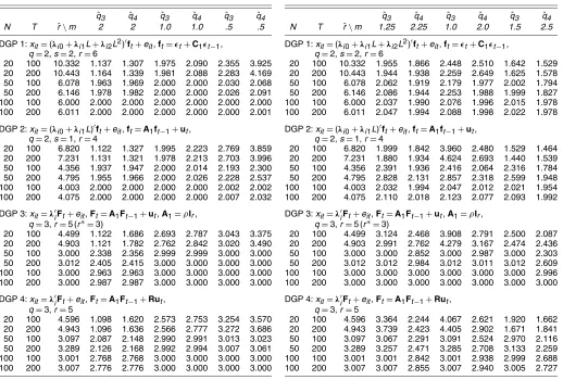
Table 1. Estimated Number of Dynamic Factors Based on the Covariance Matrix of VAR Residuals
20 100 10.332 1.137 1.307 1.975 2.090 2.355 3.925 20 200 10.443 1.164 1.339 1.981 2.088 2.283 4.169 50 100 6.078 1.963 1.969 2.000 2.000 2.030 2.068 50 200 6.146 1.978 1.982 2.000 2.000 2.026 2.091 100 100 6.000 2.000 2.000 2.000 2.000 2.000 2.000 100 200 6.011 2.000 2.000 2.000 2.000 2.000 2.001
DGP 2:xit=(λi0+λi1L)′ft+eit,ft=A1ft−1+ut,
q=2,s=1,r=4
20 100 6.820 1.122 1.327 1.995 2.223 2.769 3.859 20 200 7.231 1.131 1.321 1.978 2.213 2.703 3.996 50 100 4.356 1.937 1.947 2.000 2.014 2.193 2.300 50 200 4.795 1.955 1.966 2.000 2.026 2.228 2.537 100 100 4.003 2.000 2.000 2.000 2.000 2.002 2.002 100 200 4.075 2.000 2.000 2.000 2.000 2.007 2.032
DGP 3:xit=λ′iFt+eit,Ft=A1Ft−1+ut,A1=ρIr,
q=3,r=5 (r∗=3)
20 100 4.499 1.122 1.686 2.693 2.787 3.043 3.375 20 200 4.903 1.121 1.782 2.762 2.842 3.020 3.490 50 100 3.000 2.338 2.356 2.999 2.999 3.000 3.000 50 200 3.012 2.405 2.415 3.000 3.000 3.000 3.000 100 100 3.000 2.963 2.963 3.000 3.000 3.000 3.000 100 200 3.000 2.987 2.987 3.000 3.000 3.000 3.000
DGP 4:xit=λ′iFt+eit,Ft=A1Ft−1+Rut,
q=3,r=5
20 100 4.596 1.098 1.620 2.573 2.753 3.254 3.570 20 200 4.943 1.096 1.636 2.566 2.777 3.272 3.686 50 100 3.097 2.087 2.148 2.990 2.991 3.013 3.023 50 200 3.289 2.126 2.168 2.992 2.994 3.007 3.061 100 100 3.001 2.768 2.768 3.000 3.000 3.000 3.000 100 200 3.007 2.776 2.776 3.000 3.000 3.000 3.000
NOTE: The entries are the average values over 1,000 iterations.
addition,r∗=rfor largeT, butr∗can be less thanrfor finiteT. In all four DGPs, we assume thatλij,eit, andǫtare iid standard
normal.
For all four DGPs, the testing proceeds as follows. Given the data xit, i=1, . . . ,N, t=1, . . . ,T, the static factors are
estimated using the method of principal components with the normalization that′/N=Ir∗. The number of factors is esti-mated by the IC as done by Bai and Ng (2002). Specifically,
ˆ ing too few lags will be problematic, because uˆt will not be innovations. We report results for VAR(2); results for higher lags are similar. Given uˆt, its rˆ∗ × ˆr∗ covariance matrix is constructed. Thenqˆ3andqˆ4 are obtained withδ=.1, so that m∗=m/min[N2/5,T2/5]. The number of simulations is 1,000. Table 1 reports the average values forrˆandqˆestimated based on the covariance matrix ofuˆt. Table 2 reports the correspond-ing results based on the correlation matrix ofuˆt. The four panels correspond to four different DGPs. For all cases, the number of static factorsrˆis determined by minimizing theIC(k)fork be-tween 0 and 2r. For small values of min[N,T], the IC tends to select a large number of static factors. However, even whenrˆ∗is overestimated,qˆcan be very close toqfor suitable choice ofm.
Table 2. Estimated Number of Dynamic Factors Based on the Correlation Matrix of VAR Residuals
20 100 10.332 1.955 1.866 2.448 2.510 1.642 1.529 20 200 10.443 1.944 1.938 2.259 2.649 1.625 1.578 50 100 6.078 2.062 1.919 2.179 1.977 2.002 1.794 50 200 6.146 2.086 1.944 2.253 1.988 1.999 1.827 100 100 6.000 2.037 1.990 2.076 1.996 2.015 1.978 100 200 6.011 2.047 1.994 2.088 1.998 2.022 1.978
DGP 2:xit=(λi0+λi1L)′ft+eit,ft=A1ft−1+ut,
q=2,s=1,r=4
20 100 6.820 1.999 1.842 3.960 2.480 1.529 1.464 20 200 7.231 1.880 1.934 4.624 2.693 1.440 1.539 50 100 4.356 2.391 1.936 2.416 2.064 2.316 1.784 50 200 4.795 2.828 2.131 2.857 2.318 2.599 1.948 100 100 4.003 2.032 1.994 2.047 2.012 2.021 1.954 100 200 4.075 2.110 2.018 2.123 2.077 2.093 1.992
DGP 3:xit=λ′iFt+eit,Ft=A1Ft−1+ut,A1=ρIr,
q=3,r=5 (r∗=3)
20 100 4.499 3.124 2.468 3.908 2.791 2.500 2.087 20 200 4.903 2.991 2.762 4.279 3.167 2.474 2.436 50 100 3.000 3.000 2.852 3.000 2.987 3.000 2.303 50 200 3.012 3.012 2.984 3.012 3.011 3.012 2.609 100 100 3.000 3.000 3.000 3.000 3.000 3.000 2.996 100 200 3.000 3.000 3.000 3.000 3.000 3.000 3.000
DGP 4:xit=λ′iFt+eit,Ft=A1Ft−1+Rut,
q=3,r=5
20 100 4.596 3.364 2.244 4.067 2.621 1.920 1.662 20 200 4.943 3.739 2.423 4.405 2.902 1.671 1.841 50 100 3.097 3.067 2.291 3.091 2.524 2.970 2.116 50 200 3.289 3.257 2.471 3.285 2.708 3.133 2.259 100 100 3.001 3.001 2.842 3.001 2.938 2.999 2.688 100 200 3.007 3.007 2.855 3.007 2.940 3.005 2.727
NOTE: The entries are the average values over 1,000 iterations.
As noted earlier, when the covariance matrix is used,m=1 is suitable for bothq3andq4. But when the correlation matrix is used,mneeds to be different forq3andq4. In general, whenm is too small,qˆ is larger thanq. For all four DGPs, we find that m=1.25 works well forqˆ3 andm=2.25 works well forqˆ4 (when using correlation matrices). Betweenqˆ3andqˆ4, the for-mer tends to have better properties whenNorTis small.
5.1 Empirical Analysis: Shocks in the United States
To illustrate, we take data used by Stock and Watson (2005), which can be downloaded at http://www.princeton.edu/~ mwatson. A total of 132 monthly time series are available from 1960:1 to 2003:12. The data are transformed (by taking logs, first or second difference) as was done by Stock and Watson. The objective is to determine the number of primitive, or dy-namic, factors in this panel of data.
To get a sense of the importance of the factors in the data, we begin by determiningqˆ forr=2,3, . . . ,10.The value ofqis estimated using the correlation matrix. Almost identical results are obtained if a covariance matrix is used. But when discrep-ancy exists, the estimatedqfrom the latter method tends to be higher than that from the former method. Thus to assert thatqis larger than 2, we use a method that is less favorable to the as-sertion. In this exercise, we do not take a stand on what is the optimal number of static factors in the data. We find that for the
full sample of 528 observations, qˆ=r when r=2,3;qˆ =3, when r=4,5,6; and qˆ=4 whenr=7,8. Some of the sta-tic factors are linearly dependent in a dynamic sense. It is well known that the first two static factors in the data being analyzed are real factors. The finding thatqˆ=2 givenr=2 indicates that the first two static factors are dynamically distinct.
Next, we allow the number of static factors,rt, to be
deter-mined optimally for eacht. We use two concepts of optimal-ity. We first estimaterˆt(τ ) static factors, whereˆrt(τ )explains
the closestτ percent of the variation in the data up to timet, and then determineqˆt(τ )givenˆrt(τ )factors. Note thatrˆt(τ )is
not optimal from a statistical standpoint. However, the result of Giannone et al. (2005) thatq=2 is based on the reasoning that two dynamic factors explain 60% of the variation in 12 vari-ables. It is thus useful to consider results for cutoffs other than
τ =.6. We also determine the number of static factors using the IC. We denoted this byˆr∗t, and the corresponding number of primitive factors by q∗t. We compute all of these statistics fortranging from 133 to 528, corresponding to estimation end-ing in 1970:12 and 2003:12. We thus have 396 statistics, one statistic for everyt.
Table 3 reports the mean, minimum, and maximum of these statistics over the samples with ending dates from 1970:12 to 2003:12 (sample sizes fromT=133 toT=528).R2ˆr is the av-erage explanatory power of rˆ factors, when rˆ is chosen with cutoff of .3, .4, .5, or .6, and also optimally. The columnR2qˆ is the average explanatory power of theqˆshocks givenrˆ innova-tions.
The results indicate that four static factors explain .348 of the variation in the full-sample data, while six factors explain .438 of the variation. To explain .619 of the variation in the data would require, on average, 15 factors. When determined op-timally by IC, the data suggest that seven static factors explain
Table 3. Empirical Analysis
τ T R2
ˆ
r R
2 ˆ
q rˆ qˆ3 qˆ4
Mean .3 330.500 .323 .916 3.121 2.255 2.066 Min .3 133.000 .300 .882 3.000 2.000 1.000 Max .3 528.000 .348 1.000 4.000 4.000 3.000 Mean .4 330.500 .418 .906 5.386 3.533 3.101 Min .4 133.000 .400 .869 5.000 3.000 3.000 Max .4 528.000 .438 .967 6.000 4.000 4.000 Mean .5 330.500 .511 .902 8.833 6.068 5.210 Min .5 133.000 .500 .805 8.000 5.000 4.000 Max .5 528.000 .524 .952 10.000 7.000 6.000 Mean .6 330.500 .608 .848 13.811 8.523 7.773 Min .6 133.000 .600 .714 12.000 6.000 6.000 Max .6 528.000 .619 .908 15.000 10.000 9.000 Mean r∗ 330.500 .430 .910 5.763 3.864 3.119 Min r∗ 133.000 .239 .819 2.000 2.000 2.000 Max r∗ 528.000 .460 1.000 7.000 4.000 4.000
NOTE: This table is computed based on correlation matrix method withm=1.25 and 2.25 for
ˆ
q3andqˆ4.R2ˆris average variation inxitexplained byˆrfactors, whenˆrexplains at leastτpercent of the variation in the data up to timet.R2
ˆ
qis the percent variation inFˆtexplained byqˆprimitive shocks. The last three columns report the mean, minimum, and maximum ofˆr,qˆ3, andqˆ4over
the expanding samples with sample sizes fromT=132–528.
on average .460 of the variation in the data over the full sample, and that four dynamic factors span the seven static factors. Us-ing an alternative method but the same data, Stock and Watson (2005) found seven dynamic and static factors. In an earlier ver-sion of this article, we applied the tests to a different dataset for the sample 1960:1–1998:12. We found an average of 7 dynamic factors in 10 static factors. Thus the evidence is very compelling that the number of dynamic factors is larger than two.
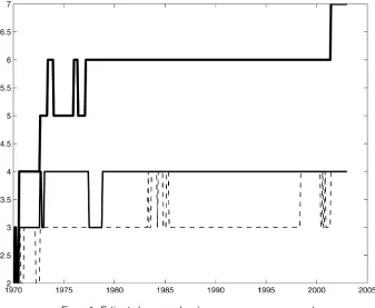
We stress once again that there is substantial variation over the sample. Figure 1 depicts time series plot ofˆrt∗,qˆ3t, andqˆ4t.
As we can see,rˆjumped from 4 to 6 around 1973 and has re-mained roughly at 6 up to 2000. On the other hand,qˆ jumped from 3 to 4 and stayed at 4 most of the time. If we had ended
Figure 1. Estimated r , q3, and q4( r; q3; q4).
Bai and Ng: Primitive Shocks in Factor Models 59
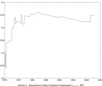
Figure 2. Importance of the Common Component ( R2).
the estimation in 2000, then we would haveˆr=6 andqˆ =4. However, in the past few years,ˆrseems to have taken another jump from 6 to 7, althoughqˆseems to have stayed at 4.
Figure 2 plots R2t, the fraction of variance in the data ex-plained by the factors up to timet. The importance of common shocks exhibit an upward trend, increasing from .25 in the early 1970s to peak at about .5 in the early 1990s. The results seem to suggest that in the early 1970s, economic fluctuations are dominated by a small number of large common shocks. More recently, the economy is hit with a larger number of smaller common shocks. Notably, for most of the sample, the stochas-tic dimension of the economy is at least four. Although the full-sample analysis obscures the fact that the optimal number of static and dynamic factors have changed over time, it remains the case that the average number of dynamic factors over the sample is more than two.
It remains to reconcile our finding thatqexceeds 2 with the result of Giannone et al. (2005). Our analysis gives the optimal number of factors for the panel of data from which the factors are extracted. Given thatN=132 series, our findings suggest that a total of 6 dynamic factors is optimal in explaining the average variation in the data. In contrast, Giannone et al. (2005) first estimated the factors from close to 200 series. They then restricted their attention to only 12 series when arriving at the conclusion thatqis 2. Their conclusion should not be taken to mean that two dynamic factors best explain the variation in the panel of data from which the factors are extracted.
To highlight the difference, we calculate the explanatory power of the common factors in the full sample for a selected number of series: IPS10 (industrial production), A0M059 (re-tail trade), A0M057 (manufacturing trade), FYFF (federal funds rate), PUNEW (CPI), and A0M224r (consumption ex-penditure). Reported are theR2from a regression ofxiton
con-stant and rˆ static factors, where xit is log first difference of
IPS10, A0M059, A0M057, and A0M224r; the first difference FYFF; and second difference of the logarithm of PUNEW. It is evident from Table 4 that the explanatory power of the factors tends to be higher for the selected series than for the panel as a whole. If we had focused on these series, then fewer static fac-tors would have been necessary. It is conceivable that four or five static factors adequately explain the selected series, which implies two or three dynamic factors.
6. CONCLUSION
This article has proposed a procedure for determining the number of primitive common shocks in a large number of se-ries. By making the link between the dynamic and the static factors precise, we arrived at a pair of tests that can determine the number of dynamic factors without having to estimate these factors themselves. This enables us to bypass the selection of many auxiliary parameters needed for estimating the spectrum. The tests are easy to compute. Our tests suggest that the num-ber of dynamic factors in the panel of 132 macroeconomic time series considered is 4.
Table 4. Explanatory Power ofˆr Factors
r
Series 1 2 3 4 5 6 7 8
ALL .172 .242 .296 .350 .393 .429 .460 .486
IPS10 .690 .723 .774 .779 .869 .869 .875 .911 A0M059 .060 .140 .149 .152 .183 .321 .321 .341 A0M057 .266 .362 .390 .397 .455 .557 .559 .562 FYFF .180 .332 .443 .445 .478 .482 .505 .515 PUNEW .008 .028 .081 .706 .711 .723 .726 .726 A0M224R .066 .142 .153 .158 .174 .227 .231 .279
NOTE: IP is industrial production, RTQ (a0m059) is retail trade, MSMTQ (a0m057) is manu-facturing trade, FYFF is Federal funds rate, PUNEW is CPI, and GMCQ (a0m224R) is consump-tion expenditure.
ACKNOWLEDGMENTS
The authors thank two anonymous referees for many con-structive comments. Financial support from the National Sci-ence Foundation (grants SES-0137084 and SES-0136923) is gratefully acknowledged.
[Received March 2005. Revised January 2006.]
REFERENCES
Anderson, T. W. (1951), “Estimating Linear Restrictions on Regression Coef-ficients for Multivariate Normal Distributions,”The Annals of Mathematical Statistics, 22, 327–351.
Bai, J. (2003), “Inferential Theory for Factor Models of Large Dimensions,”
Econometrica, 71, 135–172.
Bai, J., and Ng, S. (2002), “Determining the Number of Factors in Approximate Factor Models,”Econometrica, 70, 191–221.
Berk, K. N. (1974), “Consistent Autoregressive Spectral Estimates,”The Annals of Statistics, 2, 489–502.
Bernanke, B. (1986), “Alternative Explanations of the Money–Income Correla-tion,”Carnegie Rochester Conference on Public Policy, 25, 49–100. Bernanke, B., and Boivin, J. (2003), “Monetary Policy in a Data-Rich
Environ-ment,”Journal of Monetary Economics, 50, 525–546.
Cragg, J., and Donald, S. (1996), “On the Asymptotic Properties of LDU-Based Tests of the Rank of a Matrix,”Journal of the American Statistical Associa-tion, 91, 1301–1309.
(1997), “Inferring the Rank of a Matrix,”Journal of Econometrics, 76, 223–250.
Ding, A., and Hwang, J. (2001), “Prediction Intervals, Factor Analysis Models and High-Dimensional Empirical Linear Prediction,”Journal of the Ameri-can Statistical Association, 94, 446–455.
Forni, M., Giannone, D., Lippi, M., and Reichlin, L. (2003), “Opening the Black Box: Identifying Shocks and Propagation Mechanisms in VAR and Factor Models,” mimeo, Center for Economic Policy Research (CEPR). Forni, M., Hallin, M., Lippi, M., and Reichlin, L. (2000), “The Generalized
Dynamic Factor Model: Identification and Estimation,”Review of Economics and Statistics, 82, 540–554.
(2005), “The Generalized Dynamic Factor Model, One-Sided Esti-mation and Forecasting,”Journal of the American Statistical Association, 100, 830–840.
Forni, M., and Lippi, M. (2001), “The Generalized Dynamic Factor Model: Representation Theory,”Econometric Theory, 17, 1113–1141.
Giannone, D., Reichlin, L., and Sala, L. (2005), “Monetary Policy in Real Time,”Macroeconomic Annual, 19, 161–200.
Gill, L., and Lewbel, A. (1992), “Testing the Rank and Definiteness of Esti-mated Matrices With Applications to Factor, State-Space, and ARMA Mod-els,”Journal of the American Statistical Association, 87, 766–776. Kleibergen, F., and Paap, R. (2006), “Generalized Reduced Rank Tests Using
the Singular Value Decomposition,”Journal of Econometrics, 133, 97–126. Kuersteiner, G. (2004), “Automatic Inference for Infinite-Order Vector
Autore-gressions,”Econometric Theory, 21, 85–115.
Ratsimalahelo, Z. (2003), “Strongly Consistent Determination of the Rank of a Matrix,” unpublished manuscript, University of Franche-Comté.
Robin, J. M., and Smith, R. J. (2000), “Tests of Rank,”Econometric Theory, 16, 151–175.
Sargent, T., and Sims, C. (1977), “Business Cycle Modelling Without Pretend-ing to Have Too Much a priori Economic Theory,” inNew Methods in Busi-ness Cycle Research, ed. C. Sims, Minneapolis, MN: Federal Reserve Bank of Minneapolis, pp. 45–109.
Stock, J. H., and Watson, M. W. (2002a), “Forecasting Using Principal Compo-nents From a Large Number of Predictors,”Journal of the American Statisti-cal Association, 97, 1167–1179.
(2002b), “Macroeconomic Forecasting Using Diffusion Indexes,”
Journal of Business & Economic Statistics, 20, 147–162.
(2005), “Implications of Dynamic Factor Models for VAR Analysis,” Working Paper 11467, National Bureau of Economic Statistics.