3d simulations solid melt mixture flow melt solidification using finite volume particle method

Full Terms & Conditions of access and use can be found at

http://www.tandfonline.com/action/journalInformation?journalCode=tnst20

Journal of Nuclear Science and Technology

ISSN: 0022-3131 (Print) 1881-1248 (Online) Journal homepage: http://www.tandfonline.com/loi/tnst20

3D Simulation of Solid-Melt Mixture Flow with

Melt Solidification Using a Finite Volume Particle

Method

Rida SN MAHMUDAH , Masahiro KUMABE , Takahito SUZUKI , Liancheng

GUO & Koji MORITA

To cite this article: Rida SN MAHMUDAH , Masahiro KUMABE , Takahito SUZUKI , Liancheng GUO & Koji MORITA (2011) 3D Simulation of Solid-Melt Mixture Flow with Melt Solidification Using a Finite Volume Particle Method, Journal of Nuclear Science and Technology, 48:10, 1300-1312

To link to this article: http://dx.doi.org/10.1080/18811248.2011.9711820

Published online: 05 Jan 2012.

Submit your article to this journal

Article views: 162

View related articles

3D Simulation of Solid-Melt Mixture Flow with Melt Solidification

Using a Finite Volume Particle Method

Rida SN MAHMUDAH, Masahiro KUMABE, Takahito SUZUKI, Liancheng GUO and Koji MORITA

Department of Applied Quantum Physics and Nuclear Engineering, Kyushu University, 744 Motooka, Nishi-ku, Fukuoka 8190395, Japan

(Received January 7, 2011 and accepted in revised form May 23, 2011)

Relocation and freezing of molten core materials mixed with solid phases are among the important thermal-hydraulic phenomena in core disruptive accidents of a liquid-metal-cooled reactor (LMR). To simulate such behavior of molten metal mixed with solid particles flowing onto cold structures, a computational framework was investigated using two moving particle methods, namely, the finite volume particle (FVP) method and the distinct element method (DEM). In FVP, the fluid movement and phase changes are modeled through neighboring fluid particle interactions. For mixed-flow calculations, FVP was coupled with DEM to represent interactions between solid particles and between solid particles and the wall. A 3D computer code developed for solid-liquid mixture flows was validated by a series of pure-and mixed-melt freezing experiments using a low-melting-point alloy. A comparison between the results of experiments and simulations demonstrates that the present computational framework based on FVP and DEM is applicable to numerical simulations of solid-liquid mixture flows with freezing process under solid particle influences.

KEYWORDS: moving particle methods, finite volume particle (FVP) method, distinct element method (DEM), multiphase flow with phase change

I. Introduction

A reasonable evaluation of relocation and freezing of molten core materials mixed with various solid phases is of importance in the safety analysis of liquid-metal-cooled reactors (LMRs). In core disruptive accidents (CDAs) of an LMR, there is the hypothetical possibility of whole-core disassembly due to overheating caused by a serious transient overpower and transient undercooling accidents. These will lead to the formation of a multicomponent, multiphase flow due to the existence of a mixture of molten fuel, molten steel, fission gas, coolant vapor, refrozen fuel, broken fuel pellets, and other structural materials. The solid fuel parti-cles, which originate from early fuel pellet disruption and/or refreezing of molten fuel, could mix with the molten clad-ding material and start to flow through coolant flow chan-nels. This is one of the important issues in blockage forma-tion in the channels.

Many studies on liquid metal freezing have been conduct-ed to understand the thermal-hydraulic phenomena in CDA of LMRs. Typical experimental studies are concerned with, for example, molten jet-coolant interactions by Kondo et al.,1) thermite melt injection into an annular channel by Peppler et al.,2)and molten-metal penetration and freezing

behavior by Rahmanet al.3)_{and Hossainet al.}4)_{In the latter}

two studies,3,4) _{numerical simulations were also performed}

using a 2D Eulerian reactor safety analysis code,

SIMMER-III.5,6) _{Although their simulations show reasonably good}

agreement with observed experimental results, in general, Eulerian methods are limited in reproducing local freezing processes in detail because such methods cannot capture phase changes at the interface. In addition, the particular shape of flowing molten metal cannot be represented by mesh methods. The present study is therefore aimed at developing a reasonable computational framework that can simulate the freezing and penetration behavior of molten metal and solid mixture flows onto a metal structure.

Conventional Eulerian methods encounter difficulties in representing complex flow geometries and to directly simu-late the flow regime of mixed flows. Lagrangian methods represent one possible approach to overcome these prob-lems. Several moving particle methods, which are fully Lagrangian methods, have been developed in recent years. The earliest of these is the smoothed particle hydrodynamics

(SPH) by Monaghan,7)which was specifically developed for

compressible fluid calculations in astrophysics. The others

are the moving particle semi-implicit (MPS) method8) and

the finite volume particle (FVP) method,9) which can be

applied to incompressible multiphase flows in complex geometries. It has been validated that these are able to simulate multiphase-flow behavior with satisfactory results,

Ó

2011 Atomic Energy Society of Japan, All Rights Reserved.

_{Corresponding author, E-mail: rida@nucl.kyushu-u.ac.jp}

ARTICLE

such as fragmentation of molten metal in vapor explo-sions,10) _{water dam breakage with solid particles,}11) _{and a}

rising bubble in a stagnant liquid pool.12) _Unlike

conven-tional mesh methods, these particle methods do not need to generate computational grids. The construction of interfaces between different phases is also unnecessary because each moving particle represents each phase with specific physical properties.

In this study, a computational framework is proposed to simulate the freezing and penetration behavior of solid-liq-uid mixture flows. The developed 3D computational code is based on FVP for fluid dynamics calculations coupled with distinct element method (DEM) for solid-phase interaction calculations. To validate the fundamental models employed in fluid dynamics, as well as heat and mass transfer calcu-lations, a series of freezing experiments using pure molten metal (pure melt) was simulated using the developed 3D code. For solid-liquid mixture flows, the applicability of the present computational framework is thereby demonstrated by simulating the same for pure molten metal mixed with solid particles (mixed melt).

II. Physical Models and Numerical Methods

1. Governing Equations for Solid-Liquid Mixture Flows

The governing equations for the incompressible fluids are the Navier-Stokes equation and the continuity equation:

D u*l

and dynamic viscosity of the liquid, respectively,*f_sl is the interaction force between liquid and solid phases per unit volume, and *f_others includes other volume forces per unit volume, such as gravity and surface tension force.

The movements of solid phase are obtained by solving the following governing equations:

,m,V, andIare the translation velocity, rotation velocity, mass, volume, and inertia of a solid particle, and*F and* are the force and torque, respectively. The subscripts ‘‘col’’ and ‘‘ls’’ stand for collisions between solid phases, and interactions between solid and liquid phases, respectively. It is noted that*f_ls¼ *f_sl. The subscript ‘‘others’’ refers to other effects acting on the solid phase such as gravity.

The following energy equation that takes into account heat and mass transfer processes is solved mainly for the liquid and solid phases:

DH

Dt ¼ r ðkrTÞ þQ; ð5Þ

whereis the density,Hthe specific internal energy,T the temperature, and Q the heat transfer rate per unit volume.

The first term of the right-hand side of Eq. (5) represents the conductive heat transfer; the second term is the heat transfer at the interface between different phases.

In the present study, the surface tension force in Eq. (1) is formulated using a model based on the free surface ener-gy.13)_{The interactions between liquid and solid are evaluated}

by solving Eq. (1) even for the solid phase, which is repre-sented by solid particles.14)_{Equations (3) and (4) are solved}

using DEM. The phase-changing processes are assumed to be in nonequilibrium. In the following, we describe in detail the main physical models including FVP.

2. FVP Method

To discretize the governing equations for fluid, we choose FVP because it has been shown to be numerically stable, especially for free surface flow simulations.15)_{FVP employs}

the same concept as conventional finite volume methods. It is assumed that each particle occupies a certain volume. The control volume of one moving particle is a sphere in 3D simulations: control volume, radius of the particle control volume, and initial particle distance, respectively. According to Gauss’s law, the gradient and Laplacian operators acting on an ar-bitrary scalar functionare expressed as

r¼lim

where*n is the unit vector. As a result, in FVP, the gradient and Laplacian terms can be approximated as

hrii¼

wherehiiis the approximation ofwith respect to particle i and j*rijj is the distance between particles i and j. The

function value surf on the surface of particle i can be

estimated using a linear function:

surf¼iþ

ji

j*rijj

R: ð11Þ

The unit vector of the distance between two particles, *nij,

is defined as

The interaction surface of particle i with particle j, Sij,

can be calculated as

Sij¼

ij

n0S; ð13Þ

where the initial density, n0_{, is defined as}

n0¼X

j6¼i

ij ð14Þ

and the kernel function, ij, is defined as

ij¼sin1

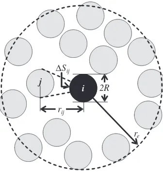
for 3D systems. If the distance between two particles is larger than the cut-off radius, the kernel function is set to zero. A schematic diagram of neighboring particles around particlei within the cut-off radius is shown inFig. 1.

Using Eqs. (11), (12), and (13), Eqs. (9) and (10) can be

Using the above gradient and Laplacian models, the gov-erning equations for fluids can be easily discretized. These equations are then solved using the combined and unified procedure (CUP) algorithm;16)a detailed explanation of this algorithm can be found in our previous study by Guoet al.14)

3. Distinct Element Method

In the present study, DEM is utilized to calculate the collision force between solid particles and between solid particles and a solid wall. The solid particles and wall par-ticles are represented by spherical parpar-ticles of equal size. The translational and rotational motions of the solid particles are calculated using time-driven DEM.17)_{Based on Eqs. (3)}

and (4), the motions of solid particle i are calculated using DEM as follows:

i are the respective vectors of position and

orientation of the center of gravity of solid particle i,F*ijis

the collision force between solid particle i and contacting solid and/or wall particlej,miandIithe respective mass and

inertia moment of solid particle i, *g is the gravitational acceleration vector, and*dcij¼ d

*

cji are vectors specifying

the position of the contact point with respect to the centers of the solid particles.

The evaluation of*Fijis presented by viscoelastic spherical

particles, while the contact force between two particlesiandj occurs due to elastic, viscous damping, and frictional effects. The particle interaction is modeled by a spring and dashpot in both the normal and tangential componentsF*n,ijandF

*

The normal component*Fn,ijof the contact force depends

on the contact geometry as well as on the physical properties of the particle’s materials and is described by Hooke’s law, taking into consideration the nonconservative viscous damp-ing response durdamp-ing the collision

F

RiþRjrepresent the reduced mass and reduced radius of particles iand j, respectively,Ei and Ejthe elasticity moduli, andviandvjthe Poisson’s ratios. In

addition, hij¼RiþRj jx

*

ijj is the overlap between

con-tacting particlesiand j, where*xijis the vector of a relative

position of the two colliding particles, *nij the unit vector

normal to the contact surface and directed towards the particle i, *vij¼ ðv

ij is the normal component of

the contact relative velocity, and n is the viscous damping

coefficient in the normal direction.

The tangential force *Ft,ij is specified by distinguishing

between tangential forces produced by static or dynamic friction:

where*tijis the unit tangential vector.

The static friction force describes friction prior to gross sliding. The most general form is based on the assumption that static friction can be calculated as the sum of elastic and viscous damping components:

where*ijis the integrated tangential displacement vector,Gi

and Gj the respective shear moduli, v

*

tangential relative velocity of the colliding particlesiandj,

and t the viscous damping coefficient in the tangential

direction.

The dynamic friction force describes friction after gross sliding and is expressed by the Coulomb law as follows:

F

whereis the friction coefficient. j

Fig. 1 Neighboring particles around particle iwithin the cut-off radius

In calculating the collision force using DEM, it is gener-ally accepted that the DEM time step size should be less than a certain critical value. The common relational form for time step size is that defined using the particle mass and stiffness:18)

where C is a constant. In general, the time step size for

DEM calculations could be much smaller than that for the fluid dynamic calculations based on the semi-implicit solution algorithm. In this study, to couple DEM with the fluid dynamic calculation, a multiple time-step scheme is applied.11)

4. Heat and Mass Transfer Model

Phase changing processes are based on a nonequilibrium model19) _{that calculates the mass transfer occurring at the}

interface between solid and liquid phases. For interfaces where no phase change is predicted, only the first term on the right-hand side of Eq. (5) is included. By the Lagrangian discretization modeled using Eq. (10), it is approximated as

hr ðkrTÞii’

where the thermal conductivitykijbetween particlesiand j

is defined as

kij¼

2kikj kiþkj

: ð27Þ

The thermal conductivity ki of particle iis simply

approxi-mated as

ki¼ ð1l,iÞks,iþl,ikl,i; ð28Þ

where ks,i and kl,i are the solid and liquid thermal

conduc-tivities of particle i, respectively, and l,i is the volume

fraction of the liquid phase in particlei.

For the interface of particle i where a phase change is

predicted, the second term on the right-hand side of Eq. (5) is calculated as

Qi;j¼aijhiðTijI TiÞ; ð29Þ

where the heat transfer coefficient depends on the thermal conductivity of particlei:

hi¼2 ki

j*rijj

ð30Þ

andTI

ij is defined as eitherT I

ij¼min½Tliq;maxðTijN;TsolÞfor

solid-liquid interface, or TI

ij¼maxðTijN;TsolÞ for solid-wall

interface, where no phase change is assumed. Tliq andTsol

are the liquidus and solidus temperatures, respectively;TN ij is

defined as the temperature for sensible heat transfer:

T_ijN¼hiTiþhjTj hiþhj

: ð31Þ

The net heat flow rate at the interface is given by

QI_i;j¼Qi;jþQj;i: ð32Þ

Once the net heat flow rate QI_ij is determined, the melting/ freezing rate can be calculated. IfQI

ij>0 and the particlei

contains a liquid phase, it will freeze partly into a solid phase; its freezing rate is calculated as

i,freezing¼

contains a solid phase, it will partially melt into a liquid phase; its melting rate is calculated as

i,melting¼

Otherwise, only sensible heat will be exchanged between particles i and j by applying T_ijN to the interface. Using Eqs. (33) and (34), the liquid and solid masses of particlei can be updated as

mn_l,iþ1¼mn_l,iþtð i,melting i,freezingÞ;

mn_s,iþ1¼mn_s,iþtð i,freezing i,meltingÞ;

ð35Þ

whereml,iandms,iare the liquid and solid masses of particle i, respectively,tis the time step size of the fluid dynamics calculation, and the superscriptnis an iterative index for the n-th time step of the calculation. Equation (35) can be used to determine the volume fraction of the liquid phase in particlei, which is necessary in evaluating its mixture ther-mal conductivity from Eq. (28).

5. Viscosity Model

In simulations of solid-liquid mixture flows, the rheolog-ical behavior has a significant influence on not only heat and mass transfer but also the dynamics of the solid and liquid during melting and freezing. In the present study, it is con-sidered by estimating the viscosity of the liquid phase with its compositional development. Based on our previous study,20)_{the viscosity model that takes into account viscosity}

changes due to phase changes is expressed using the follow-ing empirical approximation:

where app,i is the dynamic viscosity of particle i during

melting and freezing, which is in Eq. (1) instead ofl,Hliq

is the specific enthalpy at the liquidus point, and A is the rheology parameter with unit of K1_{, the value of which will}

be determined by comparing the simulation results with those of pure-melt freezing experiments. The upper limit value, max, is introduced to maintain numerical stability:

max ¼lexp

AðH¼0:375HliqÞ Cp

; ð37Þ

where H¼0:375 is the enthalpy at a liquid volume fraction

¼0:375.21)

III. Experimental Setup

Figure 2shows a schematic diagram of the experimental apparatus that was used in both pure- and mixed-melt freez-ing experiments. The apparatus consists of a melt tank and a flow channel. In the pure melt freezing experiments, we used the low-melting-point Wood’s metal as the molten metal

material. In the mixed melt experiment, a mixture of molten Wood’s metal and solid copper particles of 1 mm diameter was used to observe the effects of solid particles on melt penetration and freezing behavior. The choice of this particle material is attributed to the wettability between copper and the molten Wood’s metal.

The melt tank consists of a pot and a plug, both made of Teflon. The pot’s neck has a 4 cm length and its upper and lower inner diameters are 0.88 and 0.6 cm, respectively. The cylindrical plug is 20 cm long with a 1.4 cm outer diameter, except at the edge of the plug that contacts the upper part of the pot’s neck, where it has the same diameter as the upper neck to prevent leakage of the melt into the tank. The flow of the melt onto the flow channel is enabled by raising the plug. The pouring rate was not measured in the experiments, and hence, the pouring is assumed to occur under the free fall condition. The flow channel section is an L-shaped conduc-tion wall made of brass or copper inclined at a certain angle to enable flow along the channel. As shown in Fig. 2, the dimension of the L-shaped wall was 20:03:00:5cm in length, width, and thickness, respectively. The inclination

angle of the conduction wall is set to 15 and 30 to the

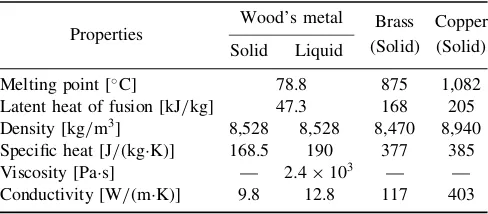
horizontal. Relevant material properties of Wood’s metal, brass, and copper are listed inTable 1.

In preparing the experiment, the melt is heated above the desired temperature in the range of 80–88_{C for melt release,}

and then transferred to the pot. When the temperature of the melt in the pot has reached the desired temperature, the plug is extracted and the melt is allowed to discharge from the pot onto the conduction wall.

During the experiments, temperatures in the pot and at the drop point onto the conduction wall (see Fig. 2) are meas-ured using thermocouples. A high-speed camera is used to record the transient behavior of the melt and to measure its penetration length along the conduction wall until the melt has completely frozen. Freezing takes about 0.2–0.8 s. A series of experiments was conducted with various param-eters,i.e., wall material, inclination angle, melt volume, and solid particle volume fraction. Conditions for the pure-and mixed-melt freezing experiments are summarized in

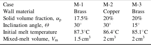
Tables 2and3, respectively.

IV. Simulation Result and Discussion

1. Simulation Setup and Boundary Conditions

In the present 3D simulations of both pure- and mixed-melt freezing experiments, the initial particle distance l was set to 1 mm, and the time step size was 0.1 ms.Figure 3

shows the channel geometry for the present simulations. With the initial particle distance of 1 mm, one moving par-ticle has a volume of 103cm3, and hence, the pure and mixed melts are represented by 1,500–2,000 moving parti-cles, depending on the melt volume. The conduction wall is

represented by an array of 200305 moving particles

corresponding to the length, width and thickness, respective-5 mm

Θ

30 mm

200 mm

Temperature recording system

High speed camera

Conduction wall melt pot

Cross-sectional view of conduction wall

plug Thermocouple

Drop point

Melt tank section

Flow channel section

Video recording system

Fig. 2 Experimental apparatus

Table 1 Material properties of Wood’s metal and solid particles

Properties

Wood’s metal _{Brass Copper}

Solid Liquid (Solid) (Solid)

Melting point [_{C] 78.8 875 1,082}

Latent heat of fusion [kJ/kg] 47.3 168 205

Density [kg/m3_{] 8,528 8,528 8,470 8,940}

Specific heat [J/(kgK)] 168.5 190 377 385

Viscosity [Pas] — 2:4103 _{— —}

Conductivity [W/(mK)] 9.8 12.8 117 403

Table 2 Conditions of pure-melt freezing experiments

Case P-1 P-2 P-3 P-4

Wall material Brass Copper Copper Copper

Inclination angle, 30 _{30 30 15}

Initial melt temperature 82.1_{C 81.6C 82.4C 82.6C}

Melt volume,Vm 2 cm3 1.5 cm3 2 cm3 2 cm3

ly. Only the first two layers of the wall particles are used as boundary particles for the fluid dynamic calculation because 2:1l is chosen for the cut-off radius re. In the heat

con-duction calculation, all the wall particles are involved in simulating the heat transfer from the melt to the wall. The present simulations did not model the heat transfer from the melt and the wall to the surrounding air because its effect on melt penetration and freezing behavior should be negligibly small over the short time period that the present experiments take.

The boundary treatment in the fluid dynamics and DEM calculations are as follows:

(1) In FVP, we have taken the zero Dirichlet condition for pressure and homogeneous Neumann condition for velocity divergences in determining the pressure for particles on the free surface.20)

(2) For the DEM simulation, a stationary plane wall de-scribing the geometrical configuration of the conduction wall is applied.

To validate the fluid dynamic models for freezing behav-ior of melt flows on a cold structure wall, the measured transient penetration length and mass distribution of frozen

molten metal are compared with simulation results. Here, the penetration length is defined as the length of the melt on the conduction wall as measured from the drop point. The mass distribution in the direction of the longitudinal length of the wall was measured for the four equal-length zones of the frozen melt. In the mixed-melt experiments, we also meas-ured the mass of solid particles in each zone. An example of the frozen melt and zone definition is presented in Fig. 4.

To validate the applicability of the fluid dynamics and the heat and mass transfer models in simulating melt flows undergoing solidification, the simulation of pure-melt freez-ing experiments was performed first. The validated models coupled with DEM were then applied to mixed-melt freezing experiments, which were performed to measure the mixture penetration and freezing behavior under the influence of the solid particles.

2. Pure Melt Freezing Simulation

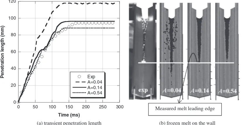
To simulate the freezing behavior of the melt on the cold structure, it is necessary to determine the rheology parameter Aappearing in Eq. (36). Its optimization was performed by carrying out certain parametric calculations of the pure-melt

freezing experiment, labeled as Case P-1. Figure 5 shows

Table 3 Conditions of mixed-melt freezing experiments

Case M-1 M-2 M-3

Wall material Brass Copper Brass

Solid volume fraction,p 17.5% 20% 20%

Inclination angle, 30 _{30 15}

Initial melt temperature 87.3_{C 86.4C 85.1C}

Mixed-melt volume,Vm 1.5 cm3 2 cm3 2 cm3

Melt Conduction wall Pot

Top view

Fig. 3 Geometrical setup of simulation

Zone 1 Zone 2 Zone 3 Zone 4

upstream downstream

Fig. 4 An example of frozen melt and zone definition

the simulation results of transient penetration length and frozen-melt shape with different rheology parameters in the range of 0.04–0.54. In the simulation results, which are indicated by the right three images, the gray and black colors indicate the conduction wall and the Wood’s metal, respec-tively. The white-colored parts, which represent the melt pot, are intentionally added to make visual comparisons easier. As can be seen in Fig. 5(b), unlike the experiment, the simulation result withA¼0:04shows an apparently disper-sive distribution of the melt on the wall. By comparing the shape of the frozen melt and the transient penetration length between the experiment and simulation, we foundA¼0:14 as a reasonable value for the rheology parameter.

To validate the applicability of the rheology model with this optimized parameter, further pure melt freezing experi-ments were simulated with a copper conduction wall, labeled as Cases P-2, P-3, and P-4.Figure 6shows the penetration length in these three cases. The simulation results for pen-etration behavior show fairly good agreement with the experiments. In the initial stages, the transient penetration length increases rapidly and then after a certain time the increase in penetration gradually reduces until the melt com-pletely freezes (no change in the penetration length). The rapid increase in penetration length in the initial stage is due to melt impacting with the conduction wall. The initial velocity of the melt in the pot is set to zero and is allowed to fall gravitationally. Given this impact velocity, melt pen-etration develops rapidly in the initial stages. However, on reaching the wall, heat transfer from the hot melt to the cold conduction wall occurs. Due to the rheological effect of the melt, the resulting temperature decrease leads to an increase in the viscosity force, which suppresses the melt velocity. The slower melt movement will lead to a smaller change in penetration length. When melt temperatures reach the freez-ing point, the melt viscosity becomes very large and the melt will completely stop penetrating along the wall. For this

reason, the heat and mass transfer model as well as the viscosity model play important roles in representing the transient behavior of melt penetration, which is reasonably reproduced by the present simulations. In addition, the simu-lated freezing time,i.e., the time taken for the melt to stop flowing on the wall, agrees well with the measurements.

The results of frozen-melt mass distribution in Cases P-1,

P-2, P-3, and P-4 are shown in Fig. 7. As can be seen in

Fig. 7, the comparison between experiments and simulations shows good agreement. All the cases indicate the same tendency for the mass distribution. Much more of the melt freezes in Zones 1 and 2, while Zone 4 yields the smallest amount of frozen mass. Approximately 70–75 vol% of the melt freeze in Zones 1 and 2 is due to the rapid heat transfer just after the melt impact on the wall and the resultant viscosity change. The remaining melt will flow along the wall with a slower velocity due to the viscosity increase.

The present simulation results for pure-melt freezing ex-periments demonstrate that the fluid dynamic models em-ployed in the developed 3D code, in particular, the heat and mass transfer models and the viscosity model, can reproduce the fundamental freezing behaviors that are observed from the melt penetration length and the frozen mass distribution under the various experimental conditions imposed.

3. Mixed-Melt Freezing Simulation

(1) DEM Effects

To validate the effectiveness of DEM in solid-liquid mix-ture freezing simulations, the simulation results of the mixed-melt freezing experiment, Case M-1, were compared with calculations using DEM and without DEM. It is noted that the calculation without DEM includes only the interac-tions between liquid and solid as the effects of solid parti-cles. Therefore, this comparison enables us to understand the effects of interactions between solid phases on melt pene-tration and freezing behavior. The properties of solid copper 0

20 40 60 80 100 120

0 50 100 150 200 250 300

Exp A=0.04 A=0.14 A=0.54

Penetration length (mm)

Time (ms)

Measured melt leading edge

(a) transient penetration length (b) frozen melt on the wall

Fig. 5 Comparison of pure-melt penetration between simulations using a different rheology parameterAand experiment (Case P-1: brass wall;¼30_;V

m¼1:5cm3)

particles used in the calculations are listed inTable 4. In the

present calculations, DEM parameters, viz. friction

coeffi-cient, and normal and tangential damping coefficients, were optimized by experimental analysis and were set to 0.2, 60, and 10 s1_{, respectively.}

The transient penetration length and mass distribution of solid particles in the frozen melt from both experiments and

simulations are compared inFig. 8, with and without DEM. The simulation result with DEM shows fairly better agree-ment than those without DEM. Without DEM, the simula-tion shows a longer penetrasimula-tion length than actual measure-ments. This is because, just after the mixed-melt begins to flow along the conduction wall, separation starts to occur for some solid particles from the bulk mixed melt. The solid particles then separately move faster than the bulk melt because they are not affected by the viscosity changes due to heat transfer. Thus, the mass of solid particles involved in the mixed melt becomes smaller than the initial solid one.

In contrast, in the simulation with DEM, the collision forces acting between solid particles and between solid par-ticles and the wall will reduce the whole momentum of solid particles, and hence, their movement would be slower than that in the simulation without DEM. As a result, the solid

0 20 40 60 80 100 120

0

Exp

Simulation

Penetration length (mm)

Time (ms) 0

20 40 60 80 100 120

0

Exp

Simulation

Penetration length (mm)

Time (ms)

0 20 40 60 80 100 120

0

Exp Simulation

Penetration length (mm)

Time (ms)

50 100 150 200 250 300 50 100 150 200 250 300

50 100 150 200 250 300

(a) Case P-2 (Θ = 30°_{; V}

m= 1.5 cm3) (b) Case P-3 (Θ = 30°; Vm= 2 cm3)

(c) Case P-4 (Θ = 15°; Vm= 2 cm3)

Fig. 6 Comparison of transient penetration length between simulation and experiment in the cases of pure melt (Cases P-2, P-3, and P-4: copper wall)

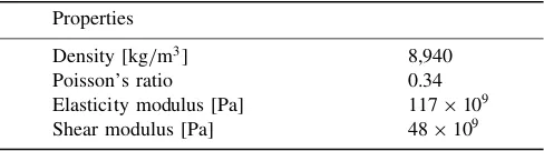
Table 4 Properties of solid copper particles

Properties

Density [kg/m3_{] 8,940}

Poisson’s ratio 0.34

Elasticity modulus [Pa] 117109

Shear modulus [Pa] 48109

particles tend to move together with the bulk melt and their separation is difficult to occur. The conclusion is that the penetration length of the mixed melt can be reasonably reproduced in simulations with DEM.

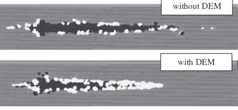
The effectiveness of DEM can also be seen from the distribution of solid particles. The solid particle distribution in the experiments and the simulation results with DEM have

a similar tendency. Figure 9shows a visual comparison of

the frozen melt on the structure surface between simulation results with and without DEM. In this figure, the black and white colors indicate Wood’s metal and the solid copper particles, respectively. The solid particles mainly gathered in Zone 4 in the simulation with DEM as well as the experi-ment, while the simulation without DEM shows the opposite result. This is caused by the separation of solid particles from the bulk of the mixed melt because, as described

before, most of the solid particles flow out of the channel without freezing with the melt.

From the above comparison of the penetration length and the mass distribution of solid particles between the simula-tion results with and without DEM, we can conclude that DEM is reasonably useful in representing the effects of solid particles mixed with molten metal on mixture freezing be-havior. Hereafter, the mixed-melt freezing flow simulations will be performed using the developed 3D code with DEM. (2) Simulation Results

The conditions in the various mixed-melt freezing simu-lations performed in the present study are summarized in

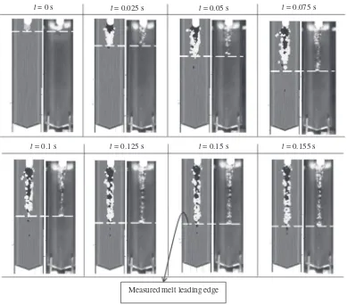
Table 3.Figure 10 shows visual comparisons of the

freez-ing process between the experiment and simulation results for Case M-1. As can be seen in this figure, where the simulation results are indicated on the left side for each 0

1 2 3 4 5 6

Exp Simulation

Melt mass (g)

Zone

0 1 2 3 4 5 6

Exp Simulation

Zone

0 1 2 3 4 5 6

1

Exp Simulation

Melt mass (g)

Zone

0 1 2 3 4 5 6

Exp Simulation

Zone (a) Case P-1 (brass wall; Θ = 30°_{; V}

m= 1.5 cm3) (b) Case P-2 (copper wall; Θ = 30°; Vm= 1.5 cm3)

(c) Case P-3 (copper wall; Θ = 30°_{; V}

m= 2 cm3) (d) Case P-4 (copper wall; Θ = 15°; Vm= 2 cm3)

2 3 4 1 2 3 4

1 2 3 4

1 2 3 4

Fig. 7 Comparison of frozen-melt mass distribution in the cases of pure melt (Case P-1, P-2, P-3, and P-4)

instant of time, the simulation and experimental results in-dicate reasonable agreement in the shape of the mixtures during freezing onto the wall. The penetration lengths of the mixture measured in the experiment are also reasonably reproduced by the present simulation, although it is hard to compare the solid particle distribution in the mixture in every instant of time qualitatively due to the limitation of photographic results in the experiment.

In the experiments, the freezing process of the mixture has a similar tendency in all the cases. When the mixed melt reaches and starts flowing on the wall, the melt will even-tually freeze and penetrate along the wall, while the solid copper particles will continue to flow until the surrounding melt freezes. Thus, Fig. 10 shows that the solid copper particles have a tendency to gather at the leading edge (Zone 4) of the frozen mixture. This is because the solid copper particles will continue to flow with the melt until it com-pletely freezes. This behavior can be explained quantitative-ly from the mass distribution of the melt and solid copper particles, as discussed below.

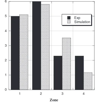
The comparisons of the mass distribution of the frozen melt between experiments and simulations are shown for Cases M-2 and M-3 inFig. 11. As can be seen in this figure, the mass distribution of the melt in each zone shows good agreement between the experiment and simulation. The dis-tribution of the melt, as has been discussed in those cases of just pure-melt freezing, concentrates mainly in Zones 1 and 2. With the copper wall (Case M-2), Zones 1 and 2 have a larger mass than the other zones, while with the brass wall (Case M-3), the mass in Zone 2 turns out to be the largest. This difference can be explained by the different heat transfer rate to the wall (copper has about 3.5 times larger thermal conductivity than brass). Regardless of the inclination of the conduction wall, the mixed melt will move not only downward but also upward just after it impacts the wall. Due to the high thermal conductivity of copper, the melt that moves in the upwards direction freezes instantly in Zone 1; in comparison with the brass wall, melt freezing develops more slowly. Thus, the melt that once moves in an upward direction will begin to flow downstream due to gravity without freezing and will eventually freeze in Zone 2.

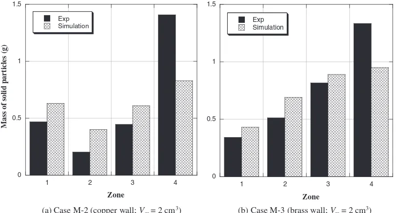
The mass distribution of solid copper particles in the frozen melt is compared between the experiment and

simu-lation results for Cases M-2 and M-3 in Fig. 12. As

dis-cussed above in Case M-1, the solid copper particles in both these cases are always found to concentrate in Zone 4, basically because these will continue to flow until the sur-rounding melt freezes. With the copper wall (Case M-2), the zone that has the second largest particle mass is Zone 1, while with the brass wall (Case M-3), this is Zone 3. This tendency can also be explained by the different heat transfer rates to the wall as discussed above. Due to the higher density of the solid copper particles than that of Wood’s metal, the solid copper particles accumulate in the lower part

0 0.2 0.4 0.6 0.8 1

1 2 3 4

Exp With DEM Without DEM

Mass of solid particles (g)

Zone 0

50 100 150 200

0 50 100 150 200 250 300

Exp With DEM Without DEM

Penetration length (mm)

Time (ms)

(a) Transient penetration length (b) Mass distribution of solid particles

Fig. 8 Comparison of mixed-melt freezing behavior between simulations with and without DEM (Case M-1: brass wall;

¼30_;

p¼17:5%,Vm¼1:5cm3)

without DEM

gray : wall; black : melt; white : solid copper particles with DEM

Fig. 9 Comparison of visualization results for frozen mixed melt between simulations with and without DEM (Case M-1)

t = 0 s t = 0.025 s t = 0.05 s t = 0.075 s

t = 0.1 s t = 0.125 s t = 0.15 s t = 0.155 s

Measured melt leading edge

Fig. 10 Comparison of visualization results for transient freezing behavior of mixed melt between simulation and experiment (Case M-1)

(a) Case M-2 (copper wall; Vm= 2 cm3) (b) Case M-3 (brass wall; Vm= 2 cm3)

0 1 2 3 4

Exp Simulation

Zone

0 1 2 3 4

1

Exp Simulation

Melt mass (g)

Zone

2 3 4 1 2 3 4

Fig. 11 Comparison of frozen-melt mass distribution in the cases of mixed melt (Cases M-2 and M-3;p¼20:0%)

of the mixture before melt release, and as a consequence, a particle-rich mixture will impact the wall first. With the copper wall, instant freezing makes the solid particles dense in Zone 1; in contrast, with the brass wall, the particle-rich mixture freezes as it reaches Zone 3, due to the relatively slower heat transfer. As a result, the frozen mixed melt contains much solid particles toward its leading edge in the downward direction.

The above three simulation results for mixed-melt freez-ing reproduce the typical characteristics of some observed mixed-melt freezing behaviors depending on the experimen-tal conditions. This demonstrates the applicability of the present fluid dynamics models coupled with DEM to the simulation of solid-liquid mixture freezing behavior under the influences of solid particles in the mixture.

V. Conclusion

In this study, to simulate the freezing behavior of solid-liquid mixture flows on a structure, a computational frame-work was proposed using the finite volume particle (FVP) method coupled with the distinct element method (DEM), which was employed to model interaction forces between solid phases. The fundamental models for the fluid-dynamics behaviors including melt rheology and heat and mass trans-fers were validated using a series of pure-melt freezing experiments. For the freezing behavior of solid-liquid mix-ture flows, the developed 3D fluid dynamics code indicates that DEM can significantly improve the simulation results. By simulating the mixed-melt freezing experiments, the val-idity of the developed code was demonstrated for various thermal and hydraulic conditions under solid particle influ-ences. It can be concluded that the developed computational framework based on the FVP method coupled with DEM can reasonably represent the freezing process of solid-liquid mixture flows on a structure.

Acknowledgements

The corresponding author, Rida SN Mahmudah, gratefully acknowledges the support from the Ministry of Education, Culture, Sports, Science and Technology of Japan under the Monkagakusho scholarship. The computation was mainly performed using the computer facilities at the Research Institute for Information Technology, Kyushu University. Finally, the authors would like to thank Mr. W. Torii, Mr. I. Miya and Mr. T. Takeda for their kind help in conducting the experiments.

Nomenclature

A: rheology parameter [K1_]

aij: contact area of particle i and j interface per unit volume

[m1_]

Cp: specific heat capacity [J/(kgK)] d

*

: vector position of contact point E: elasticity modulus [Pa] G: shear modulus [Pa] F

*

: force [N] f

*

: force per unit volume [N/m3_] g

*

: gravity [m/s2_]

H: specific enthalpy [J/kg] Hf: latent heat of fusion [J/kg]

Hliq: specific enthalpy at liquidus point [J/kg] h: heat transfer coefficient [W/(m2_K)] I: inertia of particle [kgm/s]

k: thermal conductivity [W/(mK)] l: initial particle distance [m] m: mass [kg]

n0_{: initial number density of the particles} n

*

: unit vector P: pressure [Pa]

Q: heat transfer rate per unit volume [W/m3] QI

ij: heat transfer rate at interface of particle i and j per unit

volume [W/m3_]

0 0.5 1 1.5

1 Exp Simulation

Mass of solid particles (g)

Zone

0 0.5 1 1.5

1 Exp Simulation

Zone

(a) Case M-2 (copper wall; Vm= 2 cm3) (b) Case M-3 (brass wall; Vm= 2 cm3)

2 3 4

2 3 4

Fig. 12 Comparison of solid particle mass distribution in the cases of mixed melt

R: radius of control volume [m] re: cut-off radius [m]

r: liquid particle’s position [m] S: surface of control volume [m2_]

S: interaction surface [m2_] T: temperature [K]

Tliq: liquidus temperature [K] Tsol: solidus temperature [K] t: time [s]

t

*

: unit tangential vector t: time step size [s] TI

ij: interface temperature of particleiand j[K]

u: particle’s velocity [m/s] V: volume [m3]

v

*

: contact relative velocity [m/s] x

*

: solid particle’s position [m] Greek Letters

: liquid volume fraction

: density [kg/m3_]

: dynamic viscosity coefficient [Pas]

app: dynamic viscosity coefficient during phase change [Pas] : mass transfer rate per unit volume [kg/(m3_s)]

: friction coefficient

*

: angular position of solid particle [rad]

*

: integrated tangential displacement vector

: arbitrary scalar function

: kernel function

!

*

: particle’s angular velocity [rad/s]

: viscous damping coefficient [1/s]

: Poisson’s ratio

ij: between two contacting particlesiand j l: liquid

static: static component of friction force dynamic: dynamic component of friction force

References

1) Sa. Kondo, K. Konishi, M. Isozakiet al., ‘‘Experimental study on simulated molten jet-coolant interaction,’’Nucl. Eng. Des., 204, 377–389 (1995).

2) W. Peppler, A. Kaiser, H. Will, ‘‘Freezing of a thermite melt injected into an annular channel experiments and recalcula-tions,’’Exp. Therm. Fluid Sci.,1[4], 335–346 (1988). 3) M. M. Rahman, Y. Ege, K. Morita et al., ‘‘Simulation of

molten metal freezing behavior on to a structure,’’ Nucl. Eng. Des.,238, 2706–2717 (2008).

4) M. K. Hossain, Y. Himuro, K. Moritaet al., ‘‘Simulation of molten metal penetration and freezing behavior in a seven-pin

bundle experiment,’’ Nucl. Sci. Technol., 46[8], 799–808 (2009).

5) Sa. Kondo, Y. Tobita, K. Morita et al., ‘‘SIMMER-III: An advanced computer program for LMFBR severe accident anal-ysis,’’ Proc. Int. Conf. on Design and Safety of Advanced Nuclear Power Plant(ANP ’92), Tokyo, Japan, Oct. 25–29, 1992, IV, 40.5-1 (1992).

6) Y. Tobita, Sa. Kondo, H. Yamanoet al., ‘‘Current status and application of SIMMER-III, an advanced computer program for LMFR safety analysis,’’Proc. Second Japan-Korea Symp. on Nuclear Thermal Hydraulics and Safety (NTHAS2), Fukuoka, Japan, Oct. 15–18, 2000, 65 (2000).

7) J. Monaghan, ‘‘Smoothed particle hydrodynamics,’’Rep. Prog. Phys.,68, 1703–1759 (2005).

8) S. Koshizuka, Y. Oka, ‘‘Moving-particle semi-implicit method for fragmentation of incompressible fluid,’’J. Nucl. Sci. Eng., 123, 421 (1996).

9) K. Yabushitaet al., ‘‘A finite volume particle method for an incompressible fluid flow,’’Proc. Comp. Eng. Conf.,10, 419– 421 (2005), [in Japanese].

10) S. Koshizuka, H. Ikeda, Y. Oka, ‘‘Numerical analysis of frag-mentation mechanisms in vapor explosions,’’ J. Nucl. Eng. Des.,189, 423–433 (1998).

11) S. Zhang, S. Kuwabara, T. Suzukiet al., ‘‘Simulation of solid-fluid mixture using moving particle methods,’’J. Comp. Phys., 228, 2552–2565 (2009).

12) S. Zhang, L. Guo, K. Morita et al., ‘‘Simulation of single bubble rising up in stagnant liquid pool with finite volume particle method,’’Proc. Sixth Japan-Korea Symp. on Nuclear Thermal Hydraulics and Safety (NTHAS6), Okinawa, Japan, Nov. 24–27, 2008, N6P1022 (2008).

13) M. Kondo, K. Suzuki, S. Yoshizukaet al., ‘‘Surface tension model using inter-particle force in particle method,’’FEDSM 2007 I Symposia (Part A), San Diego, USA, Jul. 30–Aug. 2, 2007, 93–98 (2007).

14) L. Guo, S. Zhang, K. Moritaet al., ‘‘Fundamental validation of the finite volume particle method for 3D sloshing dynamics,’’ to be published inInt. J. Numer. Methods Fluids.

15) S. Zhang, K. Morita, K. Fukudaet al., ‘‘A new algorithm for surface tension model in moving particle methods,’’ Int. J. Numer. Methods Fluids,55, 225–240 (2007).

16) F. Xiao, T. Yabe, M. Tajima, ‘‘An algorithm for simulating solid objects suspended in stratified flow,’’ Comput. Phys. Commun.,102, 147–160 (1997).

17) A. Dzˇiugys, B. J. Peters, ‘‘An approach to simulate the motion of spherical and non-spherical fuel particles in combustion chambers,’’Granular Matter,3[4], 231–266 (2001).

18) K. F. Malone, B. Xu, ‘‘Determination of contact parameters for discrete element method simulations of granular systems,’’

Particuology,6, 521–528 (2008).

19) K. Morita, T. Matsumoto, R. Akasakaet al., ‘‘Development of multicomponent vaporization/condensation model for a reac-tor safety analysis code SIMMER-III: Theoretical modeling and basic verification,’’Nucl. Eng. Des.,220, 224–239 (2003). 20) L. Guo, Y. Kawano, S. Zhanget al., ‘‘Numerical simulation of rheological behavior in melting metal using finite volume particle method,’’ J. Nucl. Sci. Technol., 47[11], 1011–1022 (2010).

21) D. Thomas, ‘‘Transport characteristics of suspensions,’’ J. Colloid Sci.,20, 267–277 (1965).