Fundamentals
of Digital
Image Processing
ANIL K. JAIN University of California, Davis
5
Image Transforms
5.1 INTRODUCTION
The term image transforms usually refers to a class of unitary matrices used for representing images. Just as a one-dimensional signal can be represented by an orthogonal series of basis functions, an image can also be expanded in terms of a discrete set of basis arrays called basis images. These basis images can be generated by unitary matrices. Alternatively, a given N x N image can be viewed as an N2 x 1
vector. An image transform provides a set of coordinates or basis vectors for the vector space.
For continuous functions, orthogonal series expansions provide series co efficients which can be used for any further processing or analysis of the functions. For a one-dimensional sequence {u (n), 0 ::5 n ::5 N - 1}, represented as a vector u of size N, a unitary transformation is written as
N- 1
v = Au =} v (k) = L a(k, n)u(n), Q :s; k :s; N - 1 (5.1)
where A-1 = A
*r
(unitary). This gives N - 1:::} u(n) = L v(k)a* (k, n) (5.2)
k = O
k = O
k = 1
k = 2
k = 3
k = 4
k = 5
k = 6
k = 7
... w w
Cosine
0 1 2 3 4 5 6 7
Sine
0 1 2 3 4 5 6 7
Hadamard Haar
.
0 1 2 3 4 5 6 7 0 1 2 3 4 5 6 7
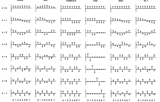
Figure 5.1 Basic vectors of the 8 x 8 transforms.
Slant
0 1 2 3 4 5 6 7
KLT
5.2 TWO-DIMENSIONAL ORTHOGONAL AND UNITARY TRANSFORMS
In the context of image processing a general orthogonal series expansion for an N x N image u (m, n) is a pair of transformations of the form discrete basis functions satisfying the properties
N - 1 called the transformed image. The orthonormality property assures that any trun cated series expansion of the form
P- I Q- 1
Up,Q (m, n) � L L v(k, l)al,, (m, n), P :s N, Q :s N (5.7)
k = O l = O
will minimize the sum of squares error
N - 1
er� = LL [u(m, n) - uP. Q (m, n)]2
m, n = O (5.8)
when the coefficients v (k, I) are given by (5.3). The completeness property assures that this error will be zero for P = Q = N (Problem 5. 1).
Separable Unitary Transforms
The number of multiplications and additions required to compute the transform coefficients v (k, I) using (5.3) is 0 (N4), which is quite excessive for practical-size images. The dimensionality of the problem is reduced to 0 (N3) when the transform is restricted to be separable, that is,
ak,1(m, n) = ak (m)b1 (n) � a(k, m)b (l, n) (5.9)
where {ak (m ), k = 0, . . . , N -1}, {b1 (n ), I = 0, . . . , N - 1} are one-dimensional complete orthonormal sets of basis vectors. Imposition of (5 .5) and (5 .6) shows that
A � {a(k, m)} and B � {b (I, n)} should be unitary matrices themselves, for example,
(5.10)
N- 1
For an M x N rectangular image, the transform pair is V = AMUAN called two-dimensional separable transformations. Unless otherwise stated, we will always imply the preceding separability when we mention two-dimensional unitary transformations. Note that (5.11) can be written as
V7 = A[AUf (5.15)
which means (5.11) can be performed by first transforming each column of U and then transforming each row of the result to obtain the rows of V.
Basis Images Equation (5.18) expresses any image U as a linear combination of the N2 matrices A;, 1, k, I = 0, .. . , N -1, which are called the basis images. Figure 5. 2 shows 8 x 8 basis images for the same set of transforms in Fig. 5.1. The transform coefficient v (k, /) is simply the inner product of the (k, /)th basis image with the given image. It is also called the projection of the image on the (k, /)th basis image. Therefore, any N x N image can be expanded in a series using a complete set of N2 basis images. If U and V are mapped into vectors by row ordering, then (5.11), (5.12), and (5.16) yield (see Section 2.8, on Kronecker products)
where
Sec. 5.2
o-= (A @ A)u � Jtu (5.20)
(5.21)
(5.22)
I
I
- .
.. ..
- .. ..
is a unitary matrix. Thus, given any unitary transform A, a two-dimensional sepa rable unitary transformation can be defined via (5.20) or (5.13).
Example 5.1
For the given orthogonal matrix A and image U
1
(
1 1)
A = yz l -1 ' u =
(; �)
the transformed image, obtained according to (5.11), is
I
(
1 1)(
1 2)(
1 1)
I(
4 6)(
1 1) (
5 -1)
V = 2 1 -1 3 4 1 -1 = 2 -2 -2 1 -1 = -2 0To obtain the basis images, we find the outer product of the columns of A* r, which gives
and similarly
* I
(
1)
I(
1 1)
Ao,0 = 2 l (1 1) = 2 l l
* I
(
1 -1)
*TAo, 1 = 2 l -l = A1,o, * I
(
1 -1)
A1,1 = 2 -l l
The inverse transformation gives
A*rVA* = �
(
1 -1 l 1)(
-2 5 -10)(
1 11 -1)
= �(
7 3 -1-1)(
1 -1 1 l)
=(
3 4 l 2)
which is U, the original image.
Kronecker Products and Dimensionality
Dimensionality of image transforms can also be studied in terms of their Kronecker product separability. An arbitrary one-dimensional transformation
(5.23) is called separable if
(5.24)
This is because (5.23) can be reduced to the separable two-dimensional trans formation
(5.25) where X and Y are matrices that map into vectors .v and..¥', respectively, by row ordering. If ._,,{, is N2 x N2 and A1 , A2 are N x N, then the number of operations required for implementing (5.25) reduces from N4 to about 2N3. The number of operations can be reduced further if A1 and A2 are also separable. Image transforms such as discrete Fourier, sine, cosine, Hadamard, Haar, and Slant can be factored as Kronecker products of several smaller-sized matrices, which leads to fast algorithms for their implementation (see Problem 5.2). In the context of image processing such matrices are also called fast image transforms.
Dimensionality of Image Transforms
The 2N3 computations for V can also be reduced by restricting the choice of A to the
fast transforms, whose matrix structure allows a factorization of the type
A = Ac!J Ac2J , . . . , A<Pl (5.26)
where AciJ , i = 1, ... ,p(p << N) are matrices with just a few nonzero entries (say r, with r<< N). Thus, a multiplication of the type y = Ax is accomplished in rpN operations. For Fourier, sine, cosine, Hadamard, Slant, and several other trans forms, p = log2 N, and the operations reduce to the order of N log2 N (or N2 log2 N for N x N images). Depending on the actual transform, one operation can be defined as one multiplication and one addition or subtraction, as in the Fourier transform, or one addition or subtraction, as in the Hadamard transform.
Transform Frequency
For a one-dimensional signal f(x), frequency is defined by the Fourier domain variable �- It is related to the number of zero crossings of the real or imaginary part of the basis function exp{j2'1T�X }. This concept can be generalized to arbitrary unitary transforms. Let the rows of a unitary matrix A be arranged so that the number of zero crossings increases with the row number. Then in the trans formation
y = Ax
the elements y (k) are ordered according to increasing wave number or transform frequency. In the sequel any reference to frequency will imply the transform frequency, that is, discrete Fourier frequency, cosine frequency, and so on. The term spatial frequency generally refers to the continuous Fourier transform fre quency and is not the same as the discrete Fourier frequency. In the case of Hadamard transform, a term called sequency is also used. It should be noted that this concept of frequency is useful only on a relative basis for a particular transform. A low-frequency term of one transform could contain the high-frequency harmonics of another transform.
The Optimum Transform
Another important consideration in selecting a transform is its performance in filtering and data compression of images based on the mean square criterion. The Karhunen-Loeve transform (KLT) is known to be optimum with respect to this criterion and is discussed in Section 5 .11.
5.3 PROPERTIES O F UNITARY TRANSFORMS
Energy Conservation and Rotation
In the unitary transformation,
v = Au
This is easily proven by noting that
N- 1 N - 1
llvll2 � k = O
L lv(k)i2=v*rv=u*rA*rAu=u*ru= L
n = O iu(n)l2 � lluii2Thus a unitary transformation preserves the signal energy or, equivalently, the length of the vector
u
in the N -dimensional vector space. This means every unitary transformation is simply a rotation of the vectoru
in the N -dimensional vector space. Alternatively, a unitary transformation is a rotation of the basis coordinates and the components ofv
are the projections ofu
on the new basis (see Problem 5 .4). Similarly, for the two-dimensional unitary transformations such as (5 .3), (5 .4), and (5 .11) to (5 . 14), it can be proven thatN- 1 N - 1
LL lu
(m, n)j2= LL Iv (k, /)12
m, n = O k, / = O
Energy Compaction and Variances of Transform Coefficients
(5 .28)
Most unitary transforms have a tendency to pack a large fraction of the average energy of the image into a relatively few components of the transform coefficients. Since the total energy is preserved, this means many of the transform coefficients will contain very little energy. If
f.Lu
andRu
denote the mean and covariance of a vectoru,
then the corresponding quantities for the transformed vector v are given byµv
�E[v] = E[Au] = AE[u] =Aµ..
Rv = E[(v - µv)(v - µ.v)*T]
= A(E[(u
-
µ.)(u - µu)*r])A*r = ARuA*r
(5 .29)
(5 .30)
The transform coefficient variances are given by the diagonal elements of
Rv ,
that iscr�(k) = [Rvh.
k= [AR. A
*1]k, kThe average energy
E[lv(k)j2]
of the transform coefficientsv(k)
tends to be un evenly distributed, although it may be evenly distributed for the input sequenceu�(k, l) = E[iv (k, l) - f.Lv(k, 1)12)
When the input vector elements are highly correlated, the transform coefficients tend to be uncorrelated. This means the off-diagonal terms of the covariance matrix Rv tend to become small compared to the diagonal elements.
With respect to the preceding two properties, the KL transform is optimum, that is, it packs the maximum average energy in a given number of transform coefficients while completely decorrelating them. These properties are presented in greater detail in Section 5 . 1 1 .
Other Properties
Unitary transforms have other interesting properties. For example, the determinant and the eigenvalues of a unitary matrix have unity magnitude. Also, the entropy of a random vector is preserved under a unitary transformation. Since entropy is a measure of average information, this means information is preserved under a unitary transformation.
Example 5.2 (Energy compaction and decorrelation)
6 E [v (O)v (l)] p Pv(O, l) = a v(O)a v(l) = 2(1 -� p2) 112
which is less in absolute value than IPI for IPI < 1 . For p = 0.95, we find Pv(O, 1) = 0.83.
Hence the correlation between the transform coefficients has been reduced. If the foregoing procedure is repeated for the 2 x 2 transform A of Example 5 .1 , then we find
The inverse transform is given by
N - 1 transformations. In image processing it is more convenient to consider the unitary
DFT, which is defined as
Future references to DFT and unitary DFT will imply the definitions of (5.39) and (5.42), respectively. The DFT is one of the most important transforms in digital signal and image processing. It has several properties that make it attractive for image processing applications.
Properties of the OFT/Unitary OFT
Let u (n) be an arbitrary sequence defined for n = 0, 1, . . . ,N - 1. A circular shift of u(n) by l, denoted by u(n -l)c , is defined as u[(n - l) modulo NJ. See Fig. 5.3 for l = 2, N = 5.
0
u(n) u[(n -2) modulo 5]
2 3 4 0 1 2 3 4
n- n - Figure 5.3 Circular shift of u(n) by 2.
The OFT and Unitary OFT matrices are symmetric. By definition the matrix F is symmetric. Therefore,
r1 = F* (5.45)
The extensions are periodic. The extensions of the DIT and unitary DIT of a sequence and their inverse transforms are periodic with period N. If for example, in the definition of (5.42) we let k take all integer values, then the sequence v (k) turns out to be periodic, that is, v(k) = v (k + N) for every k.
The OFT is the sampled spectrum of the finite sequence u(n) extended by zeros outside the interval [O, N - 1]. If we define a zero-extended sequence u(n) �
{
u(n), O :.s n :.s N - 1 (5.46)0, otherwise
then its Fourier transform is
N- 1
D(w) = 2: u(n) exp(-jwn) = 2: u (n) exp(-jwn)
n = -XI n = O
Comparing this with (5.39) we see that
v (k) = {j
Note that the unitary DIT of (5.42) would be U(2-rrk/N)IVN.
(5.47)
(5.48)
The OFT and unitary OFT of dimension N can be implemented by a fast algorithm in 0 (N log2 N) operations. There exists a class of algorithms, called the fast Fourier transform (FIT), which requires 0 (N log2 N) operations for imple menting the DIT or unitary DIT, where one operation is a real multiplication and a real addition. The exact operation count depends on N as well as the particular choice of the algorithm in that class. Most common FIT algorithms require N = 2P, where p is a positive integer.
The OFT or unitary OFT of a real sequence {x(n), n = 0, . . . ,N - 1} is conjugate symmetric about N/2. From (5.42) we obtain
N-1 N- 1
�
v(�-k)=v* (�+k),
k
= 0, . . . · 2 - 1N
(5.49)�
lv (�-k)l = lv(�+k)I
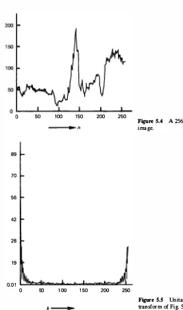
(5 .50)Figure 5.4 shows a 256-sample scan line of an image. The magnitude of its DFT is shown in Fig. 5.5, which exhibits symmetry about the point 128. If we consider the periodic extension of
v (k),
we see thatv(-k) = v(N -k)
t
u(n)
50 1 00 1 50 200 250
Figure 5.4 A 256-sample scan line of an
n image.
89
t
7056
v(k)
42
28
1 9
0.01
0 50 1 00 1 50 200 250
Figure 5.5 Unitary discrete Fourier
k transform of Fig. 5.4.
Hence the (unitary) DFT frequencies N/2 + k, k = 0, . . . , N/2 - l , are simply the negative frequencies at w = (2'ITI N)( -N 12 + k) in the Fourier spectrum of the finite sequence {u(n), 0 :5 n :5 N -1}
.
Also, from (5.39) and (5.49), we see that v(O) andv (N 12) are real, so that the N x 1 real sequence
v(O),
{
Re{v(k)}, k = 1,... , �
-1}, {
Im{v(k)}, k = 1,... , �
- 1},
v( �)
(5.51) completely defines the DFT of the real sequence u (n ). Therefore, it can be said that the DFT or unitary DFT of an N x 1 real sequence has N degrees of freedom and requires the same storage capacity as the sequence itself.The basis vectors of the unitary OFT are the orthonormal eigenvectors of any circulant matrix. Moreover, the eigenvalues of a circulant matrix are given by the OFT of its first column. Let H be an N x N circulant matrix. terms in the brackets cancel, giving the desired eigenvalue equation
[H<j>k]m = Ak<j>k(m) properties can be proven (Problem 5.9).
N-1
X2(n) = k=O L h (n - k),x1(k), 0:5n :5N-l (5.58)
then
(5.59) where DFf{x(n)}N denotes the DFf of the sequence x (n) of size N. This means we can calculate the circular convolution by first calculating the DFf of x2(n) via (5.59) and then taking its inverse DFf. Using the FFf this will take O(N log2 N) oper ations, compared to N2 operations required for direct evaluation of (5.58).
A linear convolution of two sequences can also be obtained via the FFT by imbedding it into a circular convolution. In general, the linear convolution of two sequences {h(n), n = 0, . . . , N' -1} and {x1(n), n = 0, . .. , N -1} is a se quence {x2(n), 0 :5 n :5 N' + N - 2} and can be obtained by the following algorithm: Step 1: Let M � N' + N -1 be an integer for which an FFf algorithm is available. Step 2: Define h(n) and i1(n), 0 :5 n :5 M -1, as zero extended sequences corre
sponding to h (n) and x1(n), respectively.
Step 3: Let Y1(k) = DFf{i1(n)}M, A.k = DFf{h(n)}M. Define Y2(k) = A.kY1(k), k = 0, .. . , M - 1.
Step 4: Take the inverse DFf of y2(k) to obtain i2(n). Then x2(n) = i2(n) for 0 :5 n :5 N + N ' -2.
Any circulant matrix can be diagonalized by the OFT/unitary OFT.
That is,
FHF* = A (5.60)
where A = Diag{A.k, 0 :5 k :5 N -1} and A.k are given by (5.57). It follows that if C, C1 and C2 are circulant matrices, then the following hold.
1. C1 C2 = C2 C1 , that is, circulant matrices commute.
2. c-1 is a circulant matrix and can be computed in O(N log N) operations.
3. CT, C1 + C2 , and f(C) are all circulant matrices, where f(x) is an arbitrary function of x.
5.5 THE TWO-DIMENSIONAL OFT
The two-dimensional DFf of an N x N image {u(m, n)} is a separable transform defined as
N-IN- 1
v (k, l) = L L u(m, n)Wtm W� , O :5 k, l :5 N -1 (5.61)
m=O n=O
and the inverse transform is
N - I N - 1
u(m, n) =
k�O /�O v (k, l)W,vkm w,v1n' 0 :::; m, n :::; N -1
The two-dimensional unitary OFT pair is defined as
N- I N - 1
v (k, l) =
�
m�O n�O u (m, n)W�m w�' 0 :::; k, l :::; N -1 N - I N - 1
u(m, n) =
�
k�O l�O v (k, l)W,vkm w,v1n' 0 :::; m, n :::; N - 1In matrix notation this becomes
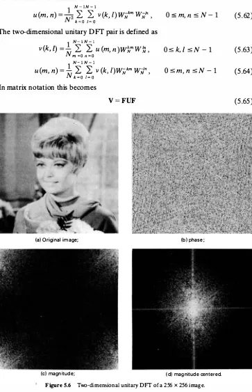
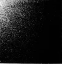
V = FUF
(a) Original image; (b) phase;
(c) magnitude; (d) magnitude centered.
Figure 5.6 Two-dimensional unitary DFT of a 256 x 256 image.
(5.62)
(5.63)
(5.64)
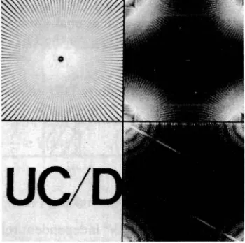
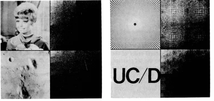
Figure 5.7 Unitary DFT of images
(a) Resolution chart; (b) its DFr;
(c) binary image;
( d) its DFr. The two parallel lines are due to the '/' sign in the binary image.
U = F*VF*
If U and V are mapped into row-ordered vectors °' and o- , respectively, then
U/ = ::F"*
0-.9" = F ® F
(5.66)
(5.67) (5.68)
The Nz x Nz matrix .9" represents the N x N two-dimensional unitary OFT. Figure
5.6 shows an original image and the magnitude and phase components of its unitary DFT. Figure 5.7 shows magnitudes of the unitary DFTs of two other images.
Properties of the Two-Dimensional OFT
The properties of the two-dimensional unitary OFT are quite similar to the one dimensional case and are summarized next.
Symmetric, unitary.
g-r
= .9",g--i
= £T* = F* ® F*Periodic extensions.
v (k + N, I + N) = v (k, /),
u(m + N, n + N) = u(m, n),
Vk, I Vm, n
(5.69)
(5.70) Sampled Fourier spectrum.
u (m, n) = 0 otherwise, then
If u(m, n) = u(m, n), 0 ::::; m, n ::::; N -1 , and
-
(
2TTk 2TT/)
U N' N = DFT{u(m, n)} = v(k, l) (5.71)
where 0 ( w1 , w2) is the Fourier transform of u (m, n ).
Fast transform. Since the two-dimensional DFT is separable, the trans formation of (5.65) is equivalent to 2N one-dimensional unitary DFfs, each of which can be performed in O (N log2 N) operations via the FFT. Hence the total number of operations is O (N2 log2 N).
Conjugate symmetry. The DFT and unitary DFT of real images exhibit conjugate symmetry, that is,
N 0 s k, l s - - 1
2 (5.72)
or
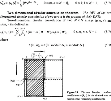
v (k, l) = v* (N - k, N -l), 0 s k, l s N - 1 (5.73) From this, it can be shown that v (k, l) has only N2 independent real elements. For example, the samples in the shaded region of Fig. 5.8 determine the complete DFT or unitary DFT (see problem 5. 10).
Basis images. The basis images are given by definition [see (5. 16) and (5.53)] :
A* _ _ _!_ {W-(km + In)
k,l -
-N N ' O s m, n s N - 1}, O s k, l s N - 1 (5.74)
Two-dimensional circular convolution theorem. The DFT of the two dimensional circular convolution of two arrays is the product of their D FTs.
Two-dimensional circular convolution of two N x N arrays h (m, n) and
u1(m, n) is defined as
N- 1 N-1
ui(m, n) = L L h(m - m ', n - n ')cu1(m ', n '), O s m, n s N - 1 (5.75) where
m' = O n' = O
k
l
( N/2) -1
N/2
h(m, n)c = h(m modulo N, n modulo N) (5.76)
N/2
Figure S.8 Discrete Fourier transform coefficients v (k, I) in the shaded area de
n n'
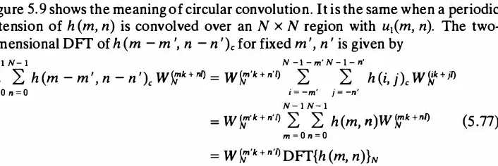
Figure 5.9 Two-dimensional circular convolution.
Figure 5.9 shows the meaning of circular convolution. It is the same when a periodic extension of h (m, n) is convolved over an N x N region with u1(m, n). The two preceding result, we obtain t
(5.78) From this and the fast transform property (page 142), it follows that an N x N circular convolution can be performed in 0 (N2 log2 N) operations. This property is also useful in calculating two-dimensional convolutions such as
Evaluating the circular convolution of h(m, n) and ii1(m, n) according to (5.75), it can be seen with the aid of Fig. 5. 9 that
x3(m, n) = u2(m, n), 0 s m, n s
2M - 2
(5.82
)This means the two-dimensional linear convolution of (5.79) can be performed in
0 (N2 log2 N) operations.
Block circulant operations. Dividing both sides of (5.77) by N and using the definition of Kronecker product, we obtain
(F @ F)9C= QJ(F @ F) (5.83)
where 9Cis doubly circulant and QJ is diagonal whose elements are given by
[QJ]kN+J,kN+J � dk,1 = DFT{h (m, n)}N , 0 s k, I s N - 1 (5.84)
Eqn. (5.83) can be written as
or (5.85)
that is, a doubly block circulant matrix is diagonalized by the two-dimensional unitary DFT. From (5.84) and the fast transform property (page 142), we conclude that a doubly block circulant matrix can be diagonalized in O (N2 log2 N) opera tions. The eigenvalues of 9C, given by the two-dimensional DFT of h (m, n), are the same as operating Ng;" on the first column of 9C. This is because the elements of the first column of 9Care the elements h(m, n) mapped by lexicographic ordering.
Block Toeplitz operations. Our discussion on linear convolution implies that any doubly block Toeplitz matrix operation can be imbedded into a double block circulant operation, which, in turn, can be implemented using the two dimensional unitary DFT.
5.6 THE COSINE TRANSFORM
The N x N cosine transform matrix C = {c(k, n)}, also called the discrete cosine trans/ orm (DCT), is defined as
{�
'k = 0, 0 s n s N - 1
c(k, n) = 1T(2n + l}k (5.86)
cos 2N , 1 s k s N -1 , 0 s n s N - 1
The one-dimensional DCT of a sequence {u (n ), 0 s n s N - 1} is defined as
where
N-l
[ (2
+ l)k]
v (k) = a(k)
n�o
u (n) cos 1T, O s k s N - 1
/:!,.
a(O) = , a(k) �
�
for 1 s k s N - 1(5.87)
822
633
443
254
t
65y(k)
- 1 25
-314
-503
50 1 00 1 50 200 250
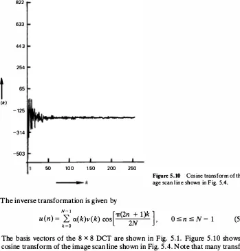
Figure 5.10 Cosine transform of the im age scan line shown in Fig. 5.4.
The inverse transformation is given by
N - l
[
1T(2n + l)k]
u (n) =
k2::o
a(k)v (k) cos2N , O :s n :s N - l (5.89)
The basis vectors of the 8 x 8 DCT are shown in Fig. 5.1. Figure 5 . 10 shows the cosine transform of the image scan line shown in Fig. 5 .4. Note that many transform coefficients are small, that is, most of the energy of the data is packed in a few transform coefficients.
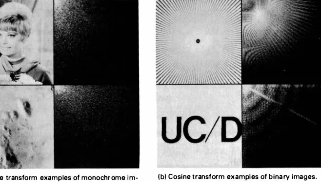
The two-dimensional cosine transform pair is obtained by substituting A = A* = C in (5. 11) and (5. 12). The basis images of the 8 x 8 two-dimensional cosine transform are shown in Fig. 5.2. Figure 5 . 1 1 shows examples of the cosine transform of different images.
Properties of the Cosine Transform
1 . The cosine transform is real and orthogonal, that is,
c
=c* � c-1
=cT
(5.90)2. The cosine transform is not the real part of the unitary DFT. This can be seen by inspection of C and the DFT matrix F. (Also see Problem 5 . 13.) However, the cosine transform of a sequence is related to the DFT of its symmetric extension (see Problem 5. 16).
(a) Cosine transform examples of monochrome im ages;
(b) Cosine transform examples of binary images.
Figure 5.11
3. The cosine transform is a fast transform. The cosine transform of a vector of N
elements can be calculated in 0 (N log2 N) operations via an N-point FIT
[19]. To show this we define a new sequence u (n) by reordering the even and
odd elements of u ( n) as
u (n) = u(2n)
l
0 :5 n :5(�)
- 1 (5.91) u(N - n - l) = u(2n + l) 'Now, we split the summation term in (5.87) into even and odd terms and use
(5.91) to obtain
{(N/2)-1 [ (4 + l)k
]
v (k) = o.(k)
n
�
o u (2n) cos 1T(N/2)-l [ (4 +
3)kJ}
+ n
�
o u (2n + 1) cos 1T n2N
{[(N/2)-l [ (4n + l)k
]
= o.(k)n
�
o u (n) cos 1T 2N(N/2)-l [ (4n +
3)kJ}
+ n
�
o u (N - n - l) cos 1T 2NChanging the index of summation in the second term to n ' = N - n - 1 and
combining terms, we obtain N -l _
[1T( 4n + 1 )k
]
v(k) = a(k) n�
o u(n) cos 2N[
N-1
= Re
a(k)e-jirk.12N n�O u(n)e-i2irkn/N]
= Re[a(k)
W�DFT{u(n)
}N
]which proves the previously stated result. For inverse cosine transform we write (5.89) for even data points as
[N-1
]
u(
2n)
= u(
2n)
�Rek�O [a(k)v(k)eiirk/2N]ei2irnk/N '
(5.93)The odd data points are obtained by noting that
u(2n
+1)
= u[
2(
N - 1-n)),
Osn s
(�)
- 1 (5.94)Therefore, if we calculate the N-point inverse FFT of the sequence
a(k)v(k)
operations. Direct algorithms that do not require FFT as an intermediate step, exp(j1Tk/2N), we can also obtain the inverse DCT in O(N logN)so that complex arithmetic is avoided, are also possible [18). The computa
tional complexity of the direct as well as the FFT based methods is about the same.
4. The cosine transform has excellent energy compaction for highly correlated
data. This is due to the following properties.
S. The basis vectors of the cosine transform (that is, rows of C) are the eigen
vectors of the symmetric tridiagonal matrix Qc , defined as
1 -a -a 0
Q� -· 1
�
0 � 1 -a
(5.95)
-a 1-a
The proof is left as an exercise.
6. The N x N cosine transform is very close to the KL transform of a first-order
stationary Markov sequence of length N whose covariance matrix is given by (2.68) when the correlation parameter pis close to
1.
The reason is that R-1 is a �mmetric tridiagonal matrix, which for a scalarJ32
�(1
- p2)/(1 + p2) anda=
p/(1 +p2)
satisfies the relation1 -pa -a
-a
1�
0
� 1
-a
1 - pa - ·(5.96)
This gives the approximation
(32 R -1 == Q, for p ==
1
(5.97)
Hence the eigenvectors of R and the eigenvectors of Q, , that is, the cosine
transform, will be quite close. These aspects are considered in greater depth in
Section
5.12
on sinusoidal transforms.This property of the cosine transform together with the fact that it is a fast
transform has made it a useful substitute for the KL transform of highly
correlated first-order Markov sequences.
5.7 THE SINE TRANSFORM
The
N
xN
sine transform matrix 'IT ={tli(k, n)},
also called thediscrete sine trans
form
(DST), is defined as(k )
.7r(k
+l)(n + 1)
1\1 'n
= smN + 1 ' Osk, n sN - 1
The sine transform pair of one-dimensional sequences is defined as(k)
=2
i( ) . TI(k + l)(n + 1) 0 s k s N - 1
v
N + 1 u n
smN + 1 '
( ) =
2
(k) . TI(k + l)(n + 1)
u n N
+
k�O smN + l ,
Osn sN- l
(5.98)
(5.99)
(5.100)
The two-dimensional sine transform pair for
N
xN
images is obtained bysubstituting A = A* = Ar = 'IT in
(5 .11)
and(5 .12).
The basis vectors and the basisimages of the sine transform are shown in Figs.
5.1
and5.2.
Figure5.12
shows thesine transform of a
255
x255
image. Once again it is seen that a large fraction of the total energy is concentrated in a few transform coefficients.Properties of the Sine Transform
1. The sine transform is real, symmetric, and orthogonal, that is,
'{f* = '{f = '{fT = '{f-1
(5.101)
Thus, the forward and inverse sine transforms are identical.
Figure 5.12 Sine transform of a 255 x
255 portion of the 256 x 256 image shown
2. The sine transform is not the imaginary part of the unitary DFT. The sine
transform of a sequence is related to the DFT of its antisymmetric extension
(see Problem 5.16).
3. The sine transform is a fast transform. The sine transform (or its inverse) of a
vector of N elements can be calculated in O(N log2N) operations via a
2(N + 1)-point FFT.
Typically this requires N + 1 =2P, that is, the fast sine transform is usually
defined for N = 3, 7, 15, 31, 63, 255, . . . . Fast sine transform algorithms that do not require complex arithmetic (or the FFT) are also possible. In fact, these algorithms are somewhat faster than the FFT and the fast cosine transform algorithms [20].
4. The basis vectors of the sine transform are the eigenvectors of the symmetric
tridiagonal Toeplitz matrix
[
1 -a
OJ
Q = - a
�
a0 -a 1 (5.102)
5. The sine transform is close to the KL transform of first order stationary
Markov sequences, whose covariance matrix is given in (2.68), when the correlation parameter p lies in the interval (-0.5, 0.5). In general it has very good to excellent energy compaction property for images.
6. The sine transform leads to a fast KL transform algorithm for Markov se
quences, whose boundary values are given. This makes it useful in many image processing problems. Details are considered in greater depth in Chapter 6 (Sections 6.5 and 6.9) and Chapter 11 (Section 11.5).
5.8 THE HADAMARD TRANSFORM
Unlike the previously discussed transforms, the elements of the basis vectors of the
Hadamard transform take only the binary values ± 1 and are, therefore, well suited
for digital signal processing. The Hadamard transform matrices, Hn , are N x N
matrices, where N � 2", n = 1, 2, 3. These can be easily generated by the core
Sec. 5.8 The Hadamard Transform
which gives
The basis vectors of the Hadamard transform can also be generated by sampling a class of functions called the
Walsh functions.
These functions also take only thebinary values ±
1
and form a complete orthonormal basis for square integrablefunctions. For this reason the Hadamard transform just defined is also called the Walsh-Hadamard transform. The number of zero crossings of a Walsh function or the number of transitions
in a basis vector of the Hadamard transform is called its
sequency.
Recall that forsinusoidal signals, frequency can be defined in terms of the zero crossings. In the
Hadamard matrix generated via
(5.104),
the row vectors are not sequency ordered.The existing sequency order of these vectors is called the
Hadamard order.
TheHadamard transform of an
N x 1
vectoru
is written asv=Hu
and the inverse transform is given byu=Hv
The two-dimensional Hadamard transform pair for
N x N
images is obtained by(a) Hadamard transforms of monochrome images. (b) Hadamard transforms of binary images.
Figure 5.13 Examples of Hadamard transforms.
images of the Hadamard transform are shown in Figs. 5.1 and 5.2. Examples of two-dimensional Hadamard transforms of images are shown in Fig. 5.13.
Properties of the Hadamard Transform
1. The Hadamard transform H is real, symmetric, and orthogonal, that is,
u = H* = HT= u-1 (5.114)
2. The Hadamard transform is a fast transform. The one-dimensional trans
formation of (5.108) can be implemented in O(N log2N) additions and sub
tractions. Since the Hadamard transform contains only ±1 values, no multiplica
tions are required in the transform calculations. Moreover, the number of additions or subtractions required can be reduced from N2 to about N log2N. This is due to the fact that Hn can be written as a product of n sparse matrices,
that is,
where
1 0
- a 1 0
H = H = Hn n '
1 0 0
0 1 1
0
n = log2N
0 0
1 1
" = v'2
-1 --1 0 0
0 0 1 -1
0 0 1 -1
Sec. 5.8 The Hadamard Transform
(5.115)
+ N
Zrows
_l
(5.116)t
N
Zrows t
Since ii contains only two nonzero terms per row, the transformation
v = ii� u = :ii:ii . . . :Hu,
n
= log2N(5.117)
n tennscan be accomplished by operating ii
n
times on u. Due to the structure of iionly N additions or subtractions are required each time ii operates on a
vector, giving a total of Nn = N log2 N additions or subtractions.
3. The natural order of the Hadamard transform coefficients turns out to be
equal to the bit reversed gray code representation of its sequency s. If the
sequency s has the binary representation bn bn _ 1 • . • b1 and if the correspond
give the forward and reverse conversion formulas for the sequency and natural ordering.
4. The Hadamard transform has good to very good energy compaction for
highly correlated images. Let {u (n ), 0 :s
n
:s N -1}
be a stationary randomTABLE 5.1 Natural Ordering versus Sequency Ordering of Hadamard
Transform Coefficients for N = 8
Gray code of s
or
Binary reverse binary Sequency binary
Natural order representation representation representation Sequency
sequence with autocorrelation
r(n), 0
::5n
::5 N- 1.
The fraction of the expected energy packed in the first N 12! sequency ordered Hadamard transform
coefficients is given by [23]
(Nl2i- l)
are simply the mean square values of the transform coefficients [Hu ]k . The
significance of this result is that 6 (N
/2i)
depends on the first2i
autocorrelations only. For j
= 1,
the fractional energy packed in the first N 12sequency ordered coefficients will be (1
+ r(l)/r(0)/2
and depends only uponthe one-step correlation p �
r(l)/r(O).
Thus for p =0.95, 97.5%
of the total energy is concentrated in half of the transform coefficients. The result of(5.120)
is useful in calculating the energy compaction efficiency of the Hadamard transform.as expected' according to (5.120).
where 0 :s p :s n - 1; q = 0, 1 for p = 0 and 1 :s q :s 2P for p ;:/= 0. For example, when N = 4, we have
k 0 1 2 3
p 0 0 1 1
q 0 1 1 2
Representing k by (p, q ), the Haar functions are defined as
L.\ 1
ho (x) = ho,o (x) = VN ' x E [0, 1].
q - l q - �
--:s x <
--2P I 2P
q - 2:sx <!L 2P 2P
otherwise for x E [O, 1]
(5.123a)
(5.123b)
The Haar transform is obtained by letting x take discrete values at m/N, m = 0,
1, .. . , N -1. For N = 8, the Haar transform is given by
Sequency
1 1 1 1 1 1 1 1 0
1 1 1 1 -1 -1 -1 -1 1
v'2 v'2 -v'2 -v'2 0 0 0 0 2
1 0 0 0 0 v'2 v'2 -v'2 -v'2 2
(5.124)
Hr =
-Vs 2 -2 0 0 0 0 0 0 2
0 0 2 -2 0 0 0 0 2
0 0 0 0 2 -2 0 0 2
0 0 0 0 0 0 2 -2 2
The basis vectors and the basis images of the Haar transform are shown in Figs. 5 .1 and 5.2. An example of the Haar transform of an image is shown in Fig. 5.14. From the structure of Hr [see ( 5 .124)] we see that the Haar transform takes differences of the samples or differences of local averages of the samples of the input vector.
Hence the two-dimensional Haar transform coefficients y (k, I), except for
k = l = 0, are the differences along rows and columns of the local averages of pixels
in the image. These are manifested as several "edge extractions" of the original image, as is evident from Fig. 5.14.
Figure S.14 Haar transform of the 256 x 256 image shown in Fig. 5.6a.
Figure S.IS Slant transform of the 256 x 256
image shown in Fig. 5.6a.
Properties of the Haar Transform
1. The Haar transform is real and orthogonal. Therefore, Hr = Hr*
Hr-1 = HrT (5.125)
2. The Haar transform is a very fast transform. On an N x 1 vector it can be
implemented in 0 (N) operations.
3. The basis vectors of the Haar matrix
are
sequency ordered.4. The Haar transform has poor energy compaction for images.
5.10 THE SLANT TRANSFORM
The N x N Slant transform matrices are defined by the recursion
where
N = 2n,
IM denotes an Mx
M identity matrix, and1
[
1 1]
S1 = Vz 1 -1
The parameters
an
andbn
are defined by the recursionswhich solve to give
( 3Nz )112
an+ 1 = 4N2 -1 '
bn+1= 4Nz-l '
(Nz- 1 )112
N = 2"Using these formulas, the
4 x 4
Slant transformation matrix is obtained asSequency
basis images of the
8 x 8
two dimensional Slant transform. Figure5.15
shows theSlant transform of a
256 x 256
image.Properties of the Slant Transform
1. The Slant transform is real and orthogonal. Therefore,
s
=
S*, s-1=
sr
2. The Sia
�
transform is a fast transform, which can beO(N
Io2N)
operations on an Nx 1
vector.3. It has ve good to excellent energy compaction for images.
(5.131)
implemented in4. The basis vectors of the Slant transform matrix S are not sequency ordered for
. = N + l
The KL transform was originally introduced as a series expansion for continuous random processes by Karhunen
[
27]
and Loeve [28]
. For random sequences Hotelling
[
26]
first studied what was called a method of principal components, which isthe discrete equivalent of the KL series expansion. Consequently, the KL transform is also called the Hotelling transform or the method of principal components.
For a real N x 1 random vector
u,
the basis vectors of the KL transform (seeSection 2. 9) are given by the orthonormalized eigenvectors of its autocorrelation
matrix R, that is,
We often work with the covariance matrix rather than the autocorrelation matrix. With µ.�
E[u],
thenRo � cov[u] �
E[(u - µ)(u - µf]
=E[uuT] - µµT
= R -µµT
(5. 136)If the vector µ. is known, then the eigenmatrix of Ro determines the KL
transform of the zero mean random process
u - µ.
In general, the KL transform ofu and
u
-µ. need not be identical.Note that whereas the image transforms considered earlier were functionally independent of the data, the KL transform depends on the (second-order) statistics of the data.
Example 5.4 (KL Transform of Markov-I Sequences)
The covariance matrix of a zero mean Markov sequence of N elements is given by (2.68). Its eigenvalues A.k and the eigenvectors cl>k are given by
1 -p2 1 - 2p COS Wk + p2
ij>k (m) = ij>(m , k)
= sin
(
wk(
m + l 1)
2 2 '
where the {wk} are the positive roots of the equation
(1 -p2) sin w
A similar result holds when N is odd. This is a transcendental equation that gives rise to nonharmonic sinusoids !J>k (m ). Figure 5.1 shows the basis vectors of this 8 x 8 KL transform for p = 0.95. Note the basis vectors of the KLT and the DCT are quite
similar. Because ij>k (m) are nonharmonic, a fast algorithm for this transform does not exist. Also note, the KL transform matrix is cllT � {ij>(k , m)}.
Example S.5
Since the unitary DFT reduces any circulant matrix to a diagonal form, it is the KL transform of all random sequences with circulant autocorrelation matrices, that is, for all periodic random sequences.
The DCT is the KL transform of a random sequence whose autocorrelation matrix R commutes with Qc of (5.95) (that is, if RQc = QcR). Similarly, the DST is the
KL transform of all random sequences whose autocorrelation matrices commute with
Q of (5.102).
KL Transform of Images
If an
N
xN
imageu(m, n)
is represented by a random field whose autocorrelationfunction is given by
E[u(m, n)u(m', n')]
=r(m, n;m', n'),
O:::::m, m', n, n' :::::N - 1
(5.139)
then the basis images of the KL transform are the orthonormalized eigenfunctions
l\lk,I
( m , n)
obtained by solving N-I N-IL L
r(m, n;m', n')l\lk,1(m', n')
m'=O n'=O
(5.140)
=
A.k,11\ik,1(m, n),
Osk,
lsN -
l,Osm, n sN -
l In matrix notation this can be written as�"1; = A.;tli;, i =
0, .. . , N2 - 1
(5.141)
where tli; is an
N2
x1
vector representation ofl\lk.i(m, n)
and � is anN2
xN2
autocorrelation matrix of the image mapped into an
N2
x1
vector u-. Thus(5.142)
If � is separable, then tfieN2
xN2
matrix 'II whose columns are {"1;} becomesseparable (see Table
2.7).
For example, lett!Jk.t (m , n) = <!>1 (m , k)<!>2 (n , l)
For row-ordered vectors this is equivalent to V = <l>jTU<l>i
The advantage in modeling the image autocorrelation by a separable function is that instead of solving the
N2 x N2 matrix eigenvalue problem of
(5.141),
only twoN x N matrix eigenvalue problems of
(5.146)
need to be solved. Since an N x Nmatrix eigenvalue problem requires 0 (N3) computations, the reduction in dimen
sionality achieved by the separable model is 0 (N6)/0 (N3) = 0 (N3), which is very
significant. Also, the transformation calculations of
(5.148)
and(5.149)
require 2N3operations compared to N4 operations required for 'i'*T U/. Example 5.6
Consider the separable covariance function for a zero mean random field
r(m ' n ; m ' ' n ') = plm-m'I pln-n'I (5.150)
The KL transform has many desirable properties, which make it optimal in many
signal processing applications. Some of these properties are discussed here. For simplicity we assume
u has zero mean and a positive definite covariance matrix R.
Decorrelation. The KL transform coefficients {v (k), k = 0,
. .
. , N- 1}
are uncorrelated and have zero mean, that is,E[v"(k)] = 0
E[v (k)v* (l)] = A.k 8(k - l)
The proof follows directly from
(5.133)
and(5.135),
sinceE(vv*1] � <l>*T E(uu1]<1> = <l>*TR<I> = A = diagonal
Sec. 5.1 1 The KL Transform
(5.151)
(5.152)
which implies the latter relation in (5. 151). It should be noted that «I» is not a
unique
matrix
with respect to this property. There could be many matrices (unitary and nonunitary) that would decorrelate the transformed sequence. For example, a lower triangular matrix «I» could be found that satisfies (5. 152).Example 5.7
The covariance matrix R of (2.68) is diagonalized by the lower triangular matrix
[
1ol
[
1 -P2
2 0]
Hence the transformation v = Lr u, will cause the sequence v(k) to be uncorrelated.
Comparing with Example 5.4, we see that L -oF cl>. Moreover, L is not unitary and the
diagonal elements of D are not the eigenvalues of R.
Basis restriction mean square error. Consider the operations in Fig. 5. 16. The vector
u
is first transformed to v. The elements of w are chosen to be the firstm
vector restricted to an
m
::5 N-dimensional subspace. The average mean squareerror between the sequences
u(n)
andz(n)
is defined as1
(N-l
)
llm �
NE
�
0lu(n)-z(n)l2
=N
Tr[E{(u-z)(u-z)*r}]
(5. 155)This quantity is called the
basis restriction error.
It is desired to find the matrices Aand B such that lm is minimized for each and every value of
m
E[1,
NJ. Thisminimum is achieved by the KL transform of
u.
Theorem 5.1. The error lm in (5 . 155) is minimum when
B = «I», AB = I (5. 156)
where the columns of «I» are arranged according to the decreasing order of the
eigenvalues of R.
Figure 5.16 KL transform basis restriction.
Using these we can rewrite (5. 155) as
lm =
�
Tr[(I -Blm A)R(I - Blm A)*r]To minimize Im we first differentiate it with respect to the elements of A and set the result to zero [see Problem 2.15 for the differentiation rules]. This gives
which yields
lm B*T = lm B*TB/m A
At m = N, the minimum value of JN must be zero, which requires
I - BA = 0 or B = A -1
Using this in (5. 160) and rearranging terms, we obtain
l s. m s. N BD, where D is a diagonal matrix. Hence, without loss of generality we can
normalize B so that B*rB = I, that is, B is a unitary matrix. Therefore, A is also
and differentiate it with respect to ai . The result giv�s a necessary condition
where at are orthonormalized eigenvectors of R. This yields
which is maximized if {at , 0
� j � m
-1} correspond to the largestm
eigenvaluesof R. Because im must be maximized for every
m,
it is necessary to arrangeAo ::: A1 ::: Az ::: · · · ::: AN-1 . Then af, the rows of A, are the conjugate transpose of the
eigenvectors of R, that is, A is the KL transform of u.
Distribution of variances. Among all the unitary transformations v = Au,
the KL transform «l>*r packs the maximum average energy in
m �
N samples of v.Threshold representation. The KL transform also minimizes
E [ m],
theexpected number of transform coefficients required, so that their energy just
exceeds a prescribed threshold (see Problem 5.26 and [33]).
A fast KL transform. In application of the KL transform to images, there are dimensionality difficulties. The KL transform depends on the statistics as well as the size of the image and, in general, the basis vectors are not known analytically. After the transform matrix has been computed, the operations for performing the transformation are quite la_rge for images.
It has been shown that certain statistical image models yield a fast KL trans form algorithm as an alternative to the conventional KL transform for images. It is based on a stochastic decomposition of an image as a sum of two random sequences.
The first random sequence
issuch that its
KLtransform
isa fast transform
and thesecond sequence, called the
boundary response,
depends only on information at theboundary points of the image. For details see Sections 6.5 and 6.9.
The rate-distortion function. Suppose a random vector u is unitary trans
A
where
8v = v -v·
represents the error in the reproduction of v. From the preceding,D is invariant under all unitary transformations. The rate-distortion function is now obtained, following Section 2.13, as
where
depend on the transform
A.
Therefore, the rateR
=
R(A)
(5.174)
(5.175)
(5.176)
(5.177)
also depends on
A.
For each fixed D,the
KLtransform achieves the minimum rate
among all unitary transforms,
that is,... b fl
1 00.00
1 0.00
Ii 1 .00
�
0 . 1 0
0
The transformation v = cl»u gives
E{[v(0)]2} = Ao = 1 + p, E{[v(1)]2} = 1 - p
1[ ( I
l + p) (
1 1 - p)]
R(cl») = 2 max 0, 2 + max 0, 2
Compare this with the case when A = I (that is, u is transmitted), which gives
O"� = O"� = 1, and
R (I) =*l-2 log 0], 0 < 0 < 1
Suppose we let 0 be small, say 0 < 1 - lpl. Then it is easy to show that R(cl») < R(I)
This means for a fixed level of distortion, the number of bits required to transmit the KLT sequence would be less than those required for transmission of the original sequence.
2
Cosine, K L
3 4 5 6 7 8 9 1 0 1 1 1 2 1 3
I ndex k
Figure 5.18 Distribution of variances of the transform coefficients (in decreasing order) of a stationary Markov sequence with N = 16, p = 0.95 (see Example 5.9).
TABLE 5.2 Variances � of Transform Coefficients of a Stationary Markov
Example 5.9 (Comparison Among Unitary Transforms for a Markov Sequence)
Consider a first-order zero mean stationary Markov sequence of length N whose
covariance matrix R is given by (2.68) with p = 0.95. Figure 5.18 shows the distribution
of variances crt of the transform coefficients (in decreasing order) for different transforms. Table 5.2 lists crt for the various transforms.
Define the normalized basis restriction error as
N - 1
where <Tl have been arranged in decreasing order.
(5. 179)
Figure 5 . 19 shows Im versus m for the various transforms. It is seen that the
cosine transform performance is indistinguishable from that of the KL transform for p = 0.95. In general it seems possible to find a fast sinusoidal transform (that is, a
transform consisting of sine or cosine functions) as a good substitute for the KL transform for different values of p as well as for higher-order stationary random
sequences (see Section 5 .12).
The mean square performance of the various transforms also depends on the dimension N of the transform. Such comparisons are made in Section 5 . 12.
Example 5.10 (Performance of Transforms on Images)
The mean square error test of the last example can be extended to actual images. Consider an N x N image u (m, n) from which its mean is subtracted out to make it zero
mean. The transform coefficient variances are estimated as
a2 (k, I) = E[lv (k, 1)12] = Iv (k, 1)12
0 2 3 4 5 6. 7 8 g 1 0 1 1 1 2 1 3 1 4 1 5 1 6 Samples retained ( m )
Figure 5.19 Performance of different unitary transforms with respect to basis
restriction errors (Jm) versus the number of basis (m) for a stationary Markov sequence with N = 16, p = 0.95.
The image transform is filtered by a
zonal mask
(Fig. 5.20) such that only a fraction of the transform coefficients are retained and the remaining ones are set to zero. Define the normalized mean square errorII lvd2 J s Ji k, l e stopband N - 1
L:L: ivd2 k, l = O
energy in stopband total energy
Figure 5.21 shows an original image and the image obtained after cosine transform zonal filtering to achieve various sample reduction ratios. Figure 5.22 shows the zonal filtered images for different transforms at a 4 : 1 sample reduction ratio. Figure 5.23
shows the mean square error versus sample reduction ratio for different transforms. Again we find the cosine transform to have the best performance.
(a) Original; (b) 4 : 1 sample reduction;
(c) 8 : 1 sample reduction; (d) 1 6 : 1 sample reduction.
Figure 5.21 Basis restriction zonal filtered images in cosine transform domain.
(a) Cosine; (b) sine;
(c) unitary OFT; (d) Hadamard;
*'
UJ U'l
::!:
"'O "'
-� n; E 0
z
1 0
B
6
4
2
1 6 B 4 2
Sample reduction ratio
Figure 5.23 Performance comparison of different transforms with respect to basis restriction zonal filtering for 256 x 256 images.
5.12 A SINUSOIDAL FAMILY OF UNITARY TRANSFORMS
This is a class of complete orthonormal sets of eigenvectors generated by the parametric family of matrices whose structure is similar to that of
a-1
[see(5.96)],
(5.180)
In fact, for
k1
=k2
=p, k3
= 0,j32
=(1 - p2)/(1
+p2),
and a =p/(1
+p2),
we haveJ(p,p,O)
=j32R-1
(5.181)
Since
R
and132a-1
have an identical set of eigenvectors, the KL transformassociated with
R
can be determined from the eigenvectors ofJ(p, p, 0).
Similarly, itcan be shown that the basis vectors of previously discussed cosine, sine, and discrete
Fourier transforms are the eigenvectors of
J(l,1,0), J(0,0,0),
andJ(l,1, -1),
respectively. In fact, several other fast transforms whose basis vectors are sinusoids
can be generated for different combinations of kl> k2, and k3• For example, for
0
:sm,
k :s N -1,
we obtain the following transforms:Other members of this family of transforms are given in
[34].
Approximation to the KL Transform
(5.182)
(5.183)
The J matrices play a useful role in performance evaluation of the sinusoidal trans
forms. For example, two sinusoidal transforms can be compared with the KL
transform by comparing corresponding J-matrix distances
.:l(kl! kz, kJ) � llJ(ki, kz, kJ) - J(p, p,
0)112
(5.184)
This measure can also explain the close performance of the DCT and the KLT. Further, it can be shown that the DCT performs better than the sine trans form for0.5
:s p :s1
and the sine transform performs better than the cosine for othervalues of p. The
J
matrices are also useful in finding a fast sinusoidal transformapproximation to the KL transform of an arbitrary random sequence whose co
variance matrix is A. If A commutes with a
J
matrix, that is, AJ = JA, then they will have an identical set of eigenvectors. The best fast sinusoidal transform may bechosen as the one whose corresponding
J
matrix minimizes thecommuting distance
llAJ
-
JAf Other uses of theJ
matrices are(1)
finding fast algorithms for inversion of banded Toeplitz matrices, ances, which are needed in transform domain processing algorithms, and(2)
efficient calculation of transform coefficient vari(3)
establishing certain useful asymptotic properties of these transforms. For details see
[34].
5.13 OUTER PRODUCT EXPANSION
AND SINGULAR VALUE DECOMPOSITION
In the foregoing transform theory, we considered an N x M image U to be a vector
in an NM-dimensional vector space. However, it is possible to represent any such image in an r-dimensional subspace where r is the rank of the matrix U.
Let the image be real and M :s N. The matrices UUT and UTU are non
negative, symmetric and have the identical eigenvalues, {>..m}. Since M :s N, there
eigenvectors {cf>m} of UTU and r orthogonal N x 1 eigenvectors {\flm} of UUT, that is,
UTUcf>m = Am cf>m ,
UUT \flm = Am \flm ,
The matrix U has the representation
u = 'II" A 112 «J>T
Equation (5.188) is called the spectral representation, the outer product expansion,
or the singular value decomposition (SVD) of U. The nonzero eigenvalues (of
which is a separable transform that diagonalizes the given image.The proof of
(5.188) is outlined in Problem 5.31.
2. The SVD transform as defined by (5.190) is not a unitary transform. This is
because W and cl> are rectangular matrices. However, we can include in «I> and W additional orthogonal eigenvectors cf>m and tflm , which satisfy Ucf>m = 0,
m = r + 1, . . . , M and UT tflm = 0, m = r + 1, . . . , N such that these matrices
are unitary and the unitary SVD transform is
(5.192)
3. The image Uk generated by the partial sum
k
Uk�
L VA:tflm <f>� ,m = l k $ r (5.193)
is the best least squares rank-k approximation of U if Am are in decreasing
order of magnitude. For any k $ r, the least squares error Let L
�
NM. Note that we can always write a two-dimensional unitary transformrepresentation as an outer product expansion in an L-dimensional space, namely,
L
is minimized for any k e [1, L] when the above expansion coincides with (5.193),
that is, when lh = Uk .
This means the energy concentrated in the trans[ orm coefficients Wi, l = 1, . . . , k is maximized by the SVD transform for the given image. Recall that the KL trans
form, maximizes the average energy in a given number of transform coefficients, the
average being taken over the ensemble for which the autocorrelation function is
defined. Hence, on an image-to-image basis, the SYD transform will concentrate
more energy in the same number of coefficients. But the SYD has to be calculated
for each image. On the other hand the KL transform needs to be calculated only
once for the whole image ensemble. Therefore, while one may be able to find a reasonable fast transform approximation of the KL transform, no such fast trans
form substitute for the SVD is expected to exist.
Although applicable in image restoration and image data compression prob
lems, the usefulness of SVD in such image processing problems is severely limited
because of large computational effort required for calculating the eigenvalues and
eigenvectors of large image matrices. However, the SVD is a fundamental result in
matrix theory that is useful in finding the generalized inverse of singular matrices and in the analysis of several image processing problems.
Example 5.11 Let
The eigenvalues ofuru are found to be A1 =
18.06,
Ai =1.94,
which give r = 2, and theSVD transform of U is
The eigenvectors are found to be
[0.5019]
<l>i =
0.8649 '
<l>i =[ 0.8649]
-0.5019
(continued on page 180)
TABLE 5.3 Summary of I mage Transforms
OFT/unitary OFT
Fast transform, most useful in digital signal processing, convolution, digital filtering, analysis of circulant and Toeplitz systems. Requires complex arithmetic. Has very good energy compaction for images. Fast transform, requires real operations, near optimal substitute for
the KL transform of highly correlated images. Useful in designing transform coders and Wiener filters for images. Has excellent energy compaction for images.
About twice as fast as the fast cosine transform, symmetric, requires real operations; yields fast KL transform algorithm which yields recursive block processing algorithms, for coding, filtering, and so
on; useful in estimating performance bounds of many image processing problems. Energy compaction for images is very good.
Faster than sinusoidal transforms, since no multiplications are required; useful in digital hardware implementations of image processing algorithms. Easy to simulate but difficult to analyze. Applications in image data compression, filtering, and design of codes. Has good energy compaction for images.
Very fast transform. Useful in feature extracton, image coding, and image analysis problems. Energy compaction is fair.
Fast transform. Has "image-like basis"; useful in image coding. Has very good energy compaction for images.
Is optimal in many ways; has no fast algorithm; useful in performance evaluation and for finding performance bounds. Useful for small size vectors e.g. , color multispectral or other feature vectors. Has the best energy compaction in the mean square sense over an ensemble.
Useful for designing fast, recursive-block processing techniques, including adaptive techniques. Its performance is better than independent block-by-block processing techniques.
Many members have fast implementation, useful in finding practical substitutes for the KL transform, analysis of Toeplitz systems, mathematical modeling of signals. Energy compaction for the optimum-fast transform is excellent.
Best energy-packing efficiency for any given image. Varies drastically from image to image; has no fast algorithm or a reasonable fast transform substitute; useful in design of separable FIR filters, finding least squares and minimum norm solutions of linear equations, finding rank of large matrices, and so on. Potential image processing applications are in image restoration, power spectrum estimation and data compression.
From above "61 is obtained via (5.191) to yield
as the best least squares rank-1 approximation of U. Let us compare this with the two dimensional cosine transform U, which is given by
[
\/2 v2 \/2][
1 2]
[
1samples of the cosine transform coefficients (show!).
5.14 SUMMARY
In this chapter we have studied the theory of unitary transforms and their proper ties. Several unitary tranforms, DFf, cosine, sine, Hadamard, Haar, Slant, KL,
sinusoidal family, fast KL, and SVD, were discussed. Table 5.3 summarizes the
various transforms and their applications.
PROBLEMS
5.1 For given P, Q show that the error er; of (5.8) is minimized when the series coefficients v (k, I) are given by (5.3). Also show that the basis images must form a complete set for er; to be zero for P = Q = N.
5.2 (Fast transforms and Kronecker separability) From (5.23) we see that the number of operations in implementing the matrix-vector product is reduced from 0 (N4) to
unitary matrices can be given this interpretation which was suggested by Good [9]. Transforms possessing this property are sometimes called Good transforms.
For the 2 x 2 transform A and the image U I
[v'3
1]
5.4 Consider the vector x and an orthogonal transform A
x =
[
;
:l
A =[
�:i:
0�:
�]
Let ao and a1 denote the columns of AT (that is, the basis vectors of A). The trans
formation y = Ax can be written as Yo = a:; x, Y1 = aI x. Represent the vector x in
Cartesian coordinates on a plane. Show that the transform A is a rotation of the
coordinates by 0 and y0 and y1 are the projections of x in the new coordinate system
(see Fig. P5.4).
Figure PS.4
5.5 Prove that the magnitude of determinant of a unitary transform is unity. Also show
that all the eigenvalues of a unitary matrix have unity magnitude.
5.6 Show that the entropy of an N x 1 Gaussian random vector u with mean p. and
covariance R. given by
is invariant under any unitary transformation.
5. 7 Consider the zero mean random vector u with covariance R. discussed in Example 5.2.
From the class of unitary transforms
Ae =
[
�:
i:
0��
s �l
v = Aeudetermine the value of 0 for which (a) the average energy compressed in Vo is
maximum and (b) the components of v are uncorrelated.
5.8 Prove the two-dimensional energy conservation relation of (5.28). 5.9 (DFT and circulant matrices)
a. Show that (5.60) follows directly from (5 .56) if cl>k is chosen as the kth column of the
unitary DFf F. Now write (5.58) as a circulant matrix operation x2 = Hx1. Take
unitary DFf of both sides and apply (5.60) to prove the circular convolution
theorem, that is, (5.59).
b. Using (5.60) show that the inverse of an N x N circulant matrix can be obtained in
0 (N log N) operations via the FFf by calculating the elements of its first column
as
Chap. 5 Problems
N- 1
[H-1]n, 0 = _!_ L w,vkn >.:;;1 = inverse DFf of {>..;;1} N k - o
c. Show that the N x 1 vector X2 = Txi , where T is N x N Toeplitz but not circulant,
can be evaluated in 0 (N log N) operations via the FFT.
5.10 Show that the N2 complex elements v(k, l) of the unitary DFT of a real sequence
{u(m, n), 0 s m, n s N - 1} can be determined from the knowledge of the partial sequence
{
v(k, O), O s k{
v(
k,�)
,os k s�}
,{
v(k, l), O s k s N - 1, 1 s / s�
- 1},
(N even)which contains only N2 nonzero real elements, in general. 5.11 a. Find the eigenvalues of the 2 x 2 doubly block circulant matrix
b. Given the arrays x1 (m, n) and X2 (m, n) as follows: n Xi (m, n) n x2 (m, n)
1 0 -1 0
1
3 4
0 -14
-10 1 2 -1 0 -1 0
m
0 1 m -1 0 1
Write their convolution X3 (m, n) = X2 (m, n) 0 X1 (m, n) as a doubly block circulant
matrix operating on a vector of size 16 and calculate the result. Verify your result by performing the convolution directly.
5.12 Show that if an image {u(m, n), 0 s m, n s N -1} is multiplied by the checkerboard pattern ( -1 r + ", then its unitary DFT is centered at (N 12, N 12). If the unitary DFT of
u(m, n) has its region of support as shown in Fig. P5.12, what would be the region of support of the unitary DFT of (-tr+" u(m, n)? Figure 5.6 shows the magnitude of the unitary DFfs of an image u (m, n) and the image ( -tr+" u (m, n ). This method can be used for computing the unitary DFT whose origin is at the center of the image matrix. The frequency increases as one moves away from the origin.
k
-N
2 N - 1
Q
i
N2
N - 1
N