Fundamentals
of Digital
Image Processing
ANIL K. JAIN University of California, Davis
11
Image Data Compression
1 1 .1 INTRODUCTION
Image data compression is concerned with minimizing the number of bits required to represent an image. Perhaps the simplest and most dramatic form of data compression is the sampling of bandlimited images, where an infinite number of pixels per unit area is reduced to one sample without any loss of information (assuming an ideal low-pass filter is available). Consequently, the number of sam ples per unit area is infinitely reduced.
Applications of data compression are primarily in transmission and storage of information. Image transmission applications are in broadcast television, remote sensing via satellite, military communications via aircraft, radar and sonar, tele conferencing, computer communications, facsimile transmission, and the like. Image storage is required for educational and business documents, medical images that arise in computer tomography (CT), magnetic resonance imaging (MRI) and digital radiology, motion pictures, satellite images, weather maps, geological sur veys, and so on. Application of data compression is also possible in the development of fast algorithms where the number of operations required to implement an algo rithm is reduced by working with the compressed data.
Image Raw Data Rates
Typical television images have spatial resolution of approximately 512 x 512 pixels per frame. At 8 bits per pixel per color channel and 30 frames per second, this translates into a rate of nearly 180 x 106 bits/s. Depending on the application, digital image raw data rates can vary from 105 bits per frame to 108 bits per frame or higher. The large-channel capacity and memory requirements (see Table l . lb) for digital image transmission and storage make it desirable to consider data compression techniques.
Data Compression versus Bandwidth Compression
The mere process of converting an analog video signal into a digital signal results in increased bandwidth requirements for transmission. For example, a 4-MHz tele vision signal sampled at Nyquist rate with 8 bits per sample would require a band width of 32 MHz when transmitted using a digital modulation scheme, such as phase shift keying (PSK), which requires 1 Hz per 2 bits. Thus, although digitized informa tion has advantages over its analog form in terms of processing flexibility, random access in storage, higher signal to noise ratio for transmission with the possibility of errrorless communication, and so on, one has to pay the price in terms of this eightfold increase in bandwidth. Data compression techniques seek to minimize this cost and sometimes try to reduce the bandwidth of the digital signal below its analog bandwidth requirements.
Image data compression methods fall into two common categories. In the first category, called predictive coding, are methods that exploit redundancy in the data. Redundancy is a characteristic related to such factors as predictability, randomness, and smoothness in the data. For example, an image of constant gray levels is fully predictable once the gray level of the first pixel is known. On the other hand, a white noise random field is totally unpredictable and every pixel has to be stored to reproduce the image. Techniques such as delta modulation and differential pulse code modulation fall into this category. In the second category, called transform coding, compression is achieved by transforming the given image into another array such that a large amount of information is packed into a small number of samples. Other image data compression algorithms exist that are generalizations or com binations of these two methods. The compression process inevitably results in some distortion because of accompanying A to D conversion as well as rejection of some relatively insignificant information. Efficient compression techniques tend to min imize this distortion. For digitized data, distortionless compression techiques are possible. Figure 11.1 gives a summary classification of various data compression techniques.
Information Rates
Raw image data rate does not necessarily represent its average information rate, which for a source with L possible independent symbols with probabilities p;,
Figure 11.1 Image data compression techniques.
i = 0, . . . , L -1, is given by the entropy
L - 1
H = -2: p; log2p; bits per symbol
i = O (11.1)
According to Shannon's noiseless coding theorem (Section 2. 13) it is possible to code, without distortion, a source of entropy H bits per symbol using H + E bits per symbol, where E is an arbitrarily small positive quantity. Then the maximum
achievable compression C, defined by
C = average bit rate of the encoded data average bit rate of the original raw data (H (B ) (ll .2)
+ E)
is B l(H + E) = B IH. Computation of such a compression ratio for images is
impractical, if not impossible. For example an N x M digital image with B bits per
pixel is one of L = 28NM possible image patterns that could occur. Thus if p;, the
probability of the ith image pattern, were known, one could compute the entropy, that is, the information rate for B bits per pixel N x M images. Then one could store all the L possible image patterns and encode the image by its address-using a suitable encoding method, which will require approximately H bits per image or
H /NM bits per pixel.
Such a method of coding is called vector quantization, or block coding [12). The main difficulty with this method is that even for small values of N and M, L can be prohibitively large; for example, for B = 8, N = M = 16 and L = 22048 = 10614•
Figure 11.2 shows a practical adaptation of this idea for vector quantization of 4 x 4
image blocks with B = 6. Each block is normalized to have zero mean and unity
variance. Using a few prototype training images, the most probable subset contain ing L ' � L images is stored. If the input block is one of these L ' blocks, it is coded by the address of the block; otherwise it is replaced by its mean value.
The entropy of an image can also be estimated from its conditional entropy. For a block of N pixels u0, ui, . . . , uN- i, with B bits per pixel and arranged in an
arbitrary order, the Nth-order conditional entropy is defined as
478
Figure 11.2 Vector quantization of images.
where each U;, i = 0, . . . , N -1, takes 28 values, and p (·,·, . . . ) represent the relevant probabilities. For 8-bit monochrome television-quality images, the zero- to second-order entropies (with nearest-neighbor ordering) generally lie in the range of 2 to 6 bits/pixel. Theoretically, for ergodic sequences, as N � oo , HN converges to
H, the per-pixel entropy. Shannon's theory tells us that the bit rate of any exact coding method can never be below the entropy H.
Subsampling, Coarse Quantization, Frame Repetition, and Interlacing
One obvious method of data compression would be to reduce the sampling rate, the number of quantization levels, and the refresh rate (number of frames per second) down to the limits of aliasing, contouring, and flickering phenomena, respectively. The distortions introduced by subsampling and coarse quantization for a given level of compression are generally much larger than the more sophisticated methods available for data compression. To avoid flicker in motion images, successive frames have to be refreshed above the critical fusion frequency (CFF), which is 50 to 60
pictures per second (Section 3.12). Typically, to capture motion a refresh rate of 25 to 30 frames per second is generally sufficient. Thus, a compression of 2 to 1 could be achieved by transmitting (or storing) only 30 frames per second but refreshing at 60 frames per second by repeating each frame. This requires a frame storage, but an image breakup or jump effect (not flicker) is often observed. Note that the frame repetition rate is chosen at 60 per second rather than 55 per second, for instance, to avoid any interference with the line frequency of 60 Hz (in the United States).
Instead of frame skipping and repetition, line interlacing is found to give better visual rendition. Each frame is divided into an odd field containing the odd line addresses and an even field containing the even line addresses; frames are transmitted alternately. Each field is displayed at half the refresh rate in frames per second. Although the jump or image breakup effect is significantly reduced by line interlacing, spatial frequency resolution is somewhat degraded because each field is a subsampled image. An appropriate increase in the scan rate (that is, lines per frame) with line interlacing gives an actual compression of about 37% for the same subjective quality at the 60 frames per second refresh rate without repetition. The success of this method rests on the fact that the human visual system has poor response for simultaneously occurring high spatial and temporal frequencies. Other interlacing techniques, such as vertical line interlacing in each field (Fig. 4.9), can reduce the data rate further without introducing aliasing if the spatial frequency spectrum does not contain simultaneously horizontal and vertical high frequencies (such as diagonal edges). Interlacing techniques are unsuitable for the display of high resolution graphics and other computer generated images that contain sharp edges and transitions. Such images are commonly displayed on a large raster (e.g. , 1024 x 1024) refreshed at 60 Hz.
1 1 .2 PIXEL CODING
In these techniques each pixel is processed independently, ignoring the inter pixel dependencies.
PCM
In PCM the incoming video signal is sampled, quantized, and coded by a suitable code word (before feeding it to a digital modulator for transmission) (Fig. 11.3). The quantizer output is generally coded by a fixed-length binary code word having B bits. Commonly, 8 bits are sufficient for monochrome broadcast or video conferencing quality images, whereas medical images or color video signals may require 10 to 12 bits per pixel.
The number of quantizing bits needed for visual display of images can be reduced to 4 to 8 bits per pixel by using companding, contrast quantization, or dithering techniques discussed in Chapter 4. Halftone techniques reduce the quantizer output to 1 bit per pixel, but usually the input sampling rate must be increased by a factor of 2 to 16. The compression achieved by these techniques is generally less than 2 : 1 .
In terms o f a mean square distortion, the minimum achievable rate b y PCM is given by the rate-distortion formula
a2 < a2 q u (11 .4)
where a� is the variance of the quantizer input and
a�
is the quantizer mean square distortion.Entropy Coding
If the quantized pixels are not uniformly distributed, then their entropy will be less than B, and there exists a code that uses less than B bits per pixel. In entropy coding the goal is to encode a block of M pixels containing MB bits with probabilities p;, i = 0, 1 , . . . , L - 1 , L = 2M8, by -log2p; bits, so that the average bit rate is
2: p; ( -log2p;) = H
i
This gives a variable-length code for each block, where highly probable blocks (or symbols) are represented by small-length codes, and vice versa. If -log2p; is not an integer, the achieved rate exceeds H but approaches it asymptotically with in creasing block size. For a given block size, a technique called Huffman coding is the most efficient fixed to variable length encoding method.
The Huffman Coding Algorithm
1. Arrange the symbol probabilities p; in a decreasing order and consider them as leaf nodes of a tree.
u(t) Sample u(nT) Zero-memory 9;(n) Digital Transmit
and hold quantizer and coder modulation
Figure 11.3 Pulse code modulation (PCM).
2. While there is more than one node:
• Merge the two nodes with smallest probability to form a new node whose
probability is the sum of the two merged nodes.
• Arbitrarily assign 1 and 0 to each pair of branches merging into a node.
3. Read sequentially from the root node to the leaf node where the symbol is located.
The preceding algorithm gives the Huffman code book for any given set of probabilities. Coding and decoding is done simply by looking up values in a table. Since the code words have variable length, a buffer is needed if, as is usually the case, information is to be transmitted over a constant-rate channel. The size of the code book is
L
and the longest code word can have as many asL
bits. These parameters become prohibitively large asL
increases. A practical version of Huff man code is called the truncated Huffman code. Here, for a suitably selected Li < L,the first
L1
symbols are Huffman coded and the remaining symbols are coded by a prefix code followed by a suitable fixed-length code.Another alternative is called the modified Huffman code, where the integer i is represented as
i = qLi + j, 0 ::=;; q ::=;;Int
[
(L
l)].
0 ::=;; j::=;;Li
-1 (11.5)The first L1 symbols are Huffman coded. The remaining symbols are coded by a prefix code representing the quotient q, followed by a terminator code, which is the same as the Huffman code for the remainder j, 0 :5 j :5
Li
-1.The long-term histogram for television images is approximately uniform, al though the short-term statistics are highly nonstationary. Consequently entropy coding is not very practical for raw image data. However, it is quite useful in predictive and transform coding algorithms and also for coding of binary data such as graphics and facsimile images.
Example 11.1
Figure 11.4 shows an example of the tree structure and the Huffman codes. The algorithm gives code words that can be uniquely decoded. This is because no code word can be a prefix of any larger-length code word. For example, if the Huffman coded bit stream is
0 0 0 1 0 1 1 0 1 0 1 1 . . .
then the symbol sequence is so s2 ss s3 .. . . A prefix code (circled elements) is obtained
by reading the code of the leaves that lead up to the first node that serves as a root for
the truncated symbols. In this example there are two prefix codes (Fig. 11.4). For the
truncated Huffman code the symbols S4, .. . , s1 are coded by a 2-bit binary code word. This code happens to be less efficient than the simple fixed length binary code in this example. But this is not typical of the truncated Huffman code.
Run-Length Coding
Consider a binary source whose output is coded as the number of Os between two successive ls, that is, the length of the runs of Os are coded. This is called run-length
Symbol
Huffman Truncated Huffman code code, L1 = 2
coding (RLC). It is useful whenever large runs of Os are expected. Such a situation occurs in printed documents, graphics, weather maps, and so on, where
p,
the probability of a 0 (representing a white pixel) is close to unity. (See Section 11.9.) Suppose the runs are coded in maximum lengths of M and, for simplicity, let M = zm - 1 . Then it will take m bits to code each run by a fixed-length code. If the successive Os occur independently, then the probability distribution of the run lengths turns out to be the geometric distributiong (l) =
{p�l -p ),
p , O s l s M - 1 l = M (11.6)Since a run length of l s M - 1 implies a sequence of l Os followed by a 1 , that is,
(1 + 1) symbols, the average number of symbols per run will be
µ = 2:
l = O (1 -p) (11 .7)
Thus it takes m bits to establish a run-length code for a sequence of µ binary
symbols, on the average. The compression achieved is, therefore,
C = � m m(l -p) = (1 -pM) (11 .8)
For p = 0.9 and M = 15 we obtain m = 4, µ = 7.94, and C = 1.985. The achieved
average rate is B. = mlµ = 0.516 bit per pixel and the code efficiency, defined as
HIB., is 0.469/0.516 = 91 %. For a given value ofp, .the optimum value of M can be
determined to give the highest efficiency. RLC efficiency can be improved further
by going to a variable length coding method such as Huffman coding for the blocks
of length m. Another alternative is to use arithmetic coding [10] instead of the RLC.
Bit-Plane Encoding [11]
I
A 256 gray-level image can be considered as a set of eight 1-bit planes, each of which
can be run-length encoded. For 8-bit monochrome images, compression ratios of 1 .5 to 2 can be achieved. This method becomes very sensitive to channel errors unless the significant bit planes are carefully protected.
1 1 .3 PREDICTIVE TECHNIQUES
Basic Principle
The philosophy underlying predictive techniques is to remove mutual redundancy between successive pixels and encode only the new information. Consider a sam
pled sequence u (m), which has been coded up to m = n -1 and let u· (n -1),
u· (n -2), . . . be the values of the reproduced (decoded) sequence. At m = n, when
u (n) arrives, a quantity u: (n), an estimate of u (n), is predicted from the previously
decoded samples u· (n - 1), u· (n -2) . . . , that is,
u· (n) = \jl(u· (n -1), u· (n -2), . . . ) (11.9)
where \jl( ·, ·, . . . ) denotes the prediction rule. Now it is sufficient to code the predic
tion error
e(n) � u (n) - u· (n) (11. 10)
If e· (n) is the quantized value of e(n), then the reproduced value of u (n) is taken as
u· (n) = u· (n) + e· (n) (11. 11)
The coding process continues recursively in this manner. This method is called
differential pulse code modulation (DPCM) or differential PCM. Figure 11.5 shows
u(n)
Figure 11.5 Differential pulse code modulation (DPCM) CODEC.
the DPCM codec (coder-decoder). Note that the coder has to calculate the re
produced sequence u· (n). The decoder is simply the predictor loop of the coder.
Rewriting (1 1. 10) as
u (n) = u· (n) + e(n)
and subtracting (11. 11) from (11. 12), we obtain
Su(n) � u(n) - u· (n) = e(n) - e· (n) = q(n)
mean square quantization error, e(n) requires fewer quantization bits than u(n).
Feedback Versus Feedforward Prediction
An important aspect of DPCM is (11.9) which says the prediction is based on the
output-the quantized samples-rather than the input-the unquantized samples. This results in the predictor being in the feedback loop around the quantizer, so that the quantizer error at a given step is fed back to the quantizer input at the next step. This has a stabilizing effect that prevents de drift and accumulation of error in the
reconstructed signal u· (n).
On the other hand, if the prediction rule is based on the past inputs (Fig. ll .6a), the signal reconstruction error would depend on all the past and present
Predictor
Figure 11.6 Feedforward coding (a) with distortion; (b) distortionless.
Image Data Compression
u0 (n)
-6 -4
5
-2 2
-5
4 6
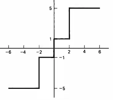
Figure 11.7 Quantizer used in Exam ple 11.2.
quantization errors in the feedforward prediction-error sequence e(n). Generally,
the mean square value of this reconstruction error will be greater than that in DPCM, as illustrated by the following example (also see Problem 11 .3).
Example 11.2
The sequence 100, 102, 120, 120, 120, 118, 116 is to be predictively coded using the previous element prediction rule, u· (n) = u· (n - 1) for DPCM and u (n) = u (n - 1) for
the feedforward predictive coder. Assume a 2-bit quantizer shown in Fig. 11.7 is used, except the first sample is quantized separately by a 7-bit uniform quantizer, giving u· (0) = u (0) = 100. The following table shows how reconstruction error builds up with
a feedforward predictive coder, whereas it tends to stabilize with the feedback system of DPCM.
Input DPCM Feedforward Predictive Coder
n u (n) u· (n) e (n) e· (n) u· (n) &u(n) u (n) E(n) E0 (n) u· (n) &u(n)
0 100 100 0 100 0
1 102 100 2 1 101 1 100 2 1 101 1
Edge --> 2 120 101 19 5 106 14 102 18 5 106 14
3 120 106 14 5 111 9 120 0 - 1 105 15
4 120 111 9 5 116 4 120 0 -1 104 16
5 118 116 2 117 120 -2 -5 99 19
Distortionless Predictive Coding
In digital processing the input sequence u(n) is generally digitized at the source
itself by a sufficient number of bits (typically 8 for images). Then, u(n) may be
considered as an integer sequence. By requiring the predictor outputs to be integer values, the prediction error sequence will also take integer values and can be entropy coded without distortion. This gives a distortionless predictive codec (Fig. 1 1.6b ), whose minimum achievable rate would be equal to the entropy of the
prediction-error sequence e(n).
Performance Analysis of DPCM
Denoting the mean square values of quantization error q(n) and the prediction
error e(n) by CJ� and CJ� , respectively, and noting that (11 .13) implies
E[(8u(n))2] = CJ� (11. 14)
the minimum achievable rate by DPCM is given by the rate-distortion formula [see
(2. 116)]
RvPcM =
�
log2(:D
bits/pixel (11.15)In deducing this relationship, we have used the fact that common zero memory quantizers (for arbitrary distributions) do not achieve a rate lower than the Shannon quantizer for Gaussian distributions (see Section 4.9). For the same distortion
CJ
�
5 CJ� , the reduction in DPCM rate compared to PCM is [see (11.4)]RPcM - RvPcM =
�
log2(:D
= log10(:D
bits/pixel (11 . 16)This shows the achieved compression depends on the reduction of the variance ratio
(CJ� /CJ�), that is, on the ability to predict u (n) and, therefore, on the intersample
redundancy in the sequence. Also, the recursive nature of DPCM requires that the
predictor be causal. For minimum prediction-error variance, the optimum predictor
is the conditional mean E[u(n)ju· (m), m 5 n -1]. Because of the quantizer, this is
a nonlinear function and is difficult to determine even when u (n) is a stationary
Gaussian sequence. The optimum feedforward predictor is linear and shift invariant for such sequences, that is,
u (n) = <l>(u(n - 1), . . . ) = L a (k)u(n - k) (11.17) k
If the feedforward prediction error E(n) has variance 132, then
132 5 CJ� (11 . 18)
This is true because u· (n) is based on the quantization noise contammg
samples { u· ( m ), m 5 n} and could never be better than u ( n ). As the number of
quantization levels is increased to infinity, CJ� will approach 132. Hence, a lower
bound on the rate achievable by DPCM is
(11. 19)
When the quantization error is small, RvPcM approaches Rmin • This expression is
useful because· it is much easier to evaluate �2 than CJ� in (11. 15), and it can be used
to estimate the achievable compression. The SNR corresponding to CJ� is given by
CJ2 CJ2 CJ2
(SNR)vPcM = 10 log10 10 log1o 5 10 log10 132 (11 .20)
where f(B) is the quantizer mean square distortion function for a unit variance
input and B quantization bits. For equal number of bits used, the gain in SNR of
DPCM over PCM is
[CT�]
(SNR)vPcM - (SNR)PcM = 10 log10CT�
:5 10 log10 132 dB (11 .21)which is proportional to the log of the variance ratio
(CT�
/132). Using (11 . 16) we notethat the increase in SNR is approximately 6 (RPcM - RvPcM) dB, that is, 6 dB per bit
of available compression.
From these measures we see that the performance of predictive coders depends on the design of the predictor and the quantizer. For simplicity, the predic tor is designed without considering the quantizer effects. This means the prediction
rule deemed optimum for u (n) is applied to estimate u· (n). For example, if u (n) is
given by (11. 17) then the DPCM predictor is designed as
u· (n) = <l>(u· (n - 1), u· (n - 2), . . . ) = 2: a (k)u· (n - k) (11.22) k
In two (or higher) dimensions this approach requires finding the optimum causal prediction rules. Under the mean square criterion the minimum variance causal
representations can be used directly. Note that the DPCM coder remains nonlinear
even with the linear predictor of (11.22). However, the decoder will now be a linear filter. The quantizer is generally designed using the statistical properties of the
innovations sequence e(n), which can be estimated from the predictor design.
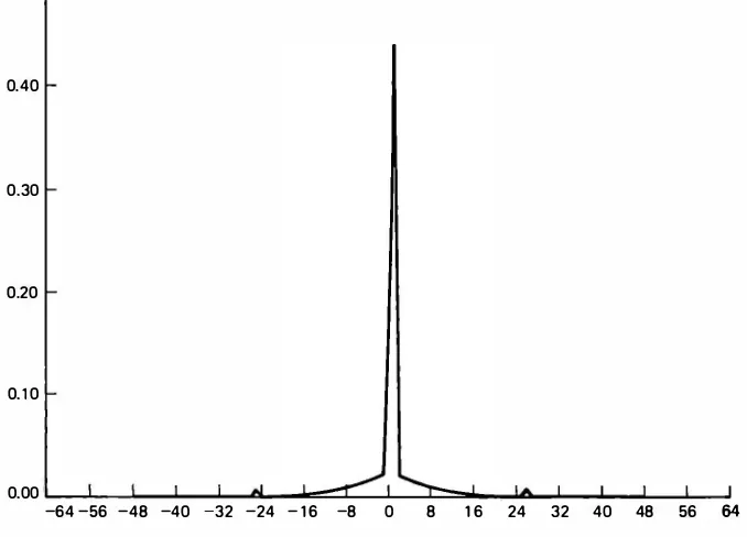
Figure 1 1 .8 shows a typical prediction error signal histogram. Note the prediction
0.50
0.40
0.30
0.20
0.1 0
0.00
-64 -56 -48 -40 -32 -24 - 1 6 -8 0 8 1 6 24 32 40 48 56 64
Figure 11.8 Predictions = error histogram.
error takes large values near the edges. Often, the prediction error is modeled as a zero mean uncorrelated sequence with a Laplacian probability distribution, that is,
1
(-v'2 )
p (E) = 132 exp (11.23)
where 132 is its variance. The quantizer is generally chosen to be either the Lloyd Max (for a constant bit rate at the output) or the optimum uniform quantizer (followed by an entropy coder to minimize the average rate). Practical predictive codecs differ with respect to realizations and the choices of predictors and quantizers. Some of the common classes of predictive codecs for images are de scribed next.
Delta Modulation
Delta modulation (DM) is the simplest of the predictive coders. It uses a one-step delay function as a predictor and a 1-bit quantizer, giving a 1-bit representation of the signal. Thus
u· (n) = u· (n
-
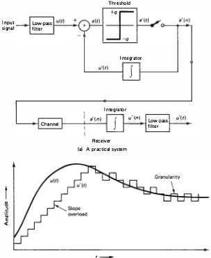
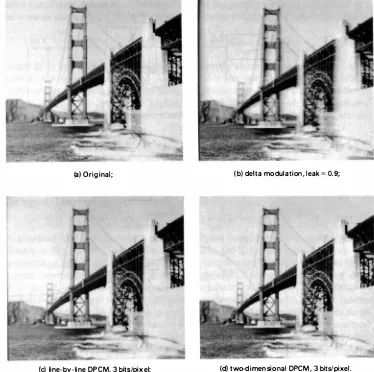
1), e(n) = u (n) - u· (n - 1) (11 .24) A practical DM system, which does not require sampling of the input signal, is shown in Fig. ll.9a. The predictor integrates the quantizer output, which is a sequence of binary pulses. The receiver is a simple integrator. Figure 11.9b shows typical input-output signals of a delta modulator. Primary limitations of delta modulation are (1) slope overload, (2) granularity noise, and (3) instability to channel errors. Slope overload occurs whenever there is a large jump or discon tinuity in the signal, to which the quantizer can respond only in several delta steps. Granularity noise is the steplike nature of the output when the input signal is almost constant. Figure 11. lOb shows the blurring effect of slope overload near the edges and the granularity effect in the constant gray-level background.Both of these errors can be compensated to a certain extent by low-pass filtering the input and output signals. Slope overload can also be reduced by in creasing the sampling rate, which will reduce the interpixel differences. However, the higher sampling rate will tend to lower the achievable compression. An alterna tive for reducing granularity while retaining simplicity is to go to a tristate delta modulator. The advantage is that a large number (65 to 85%) of pixels are found to be in the level, or 0, state, whereas the remaining pixels are in the ± 1 states. Huffman coding the three states or run-length coding the 0 states with a 2-bit code for the other states yields rates around 1 bit per pixel for different images [14].
The reconstruction filter, which is a simple integrator, is unstable. Therefore, in the presence of channel errors, the receiver output can accumulate large errors. It can be stabilized by attenuating the predictor output by a positive constant p < 1
(called leak). This will, however, not retain the simple realization of Pig. 11.9a. For delta modulation of images, the signal is generally presented line by line and no advantage is taken of the two-dimensional correlation in the data. When each scan line of the image is represented by a first-order AR process (after subtracting the mean),
I nput signal
t
Q) -0-� a. E <!
Low-pass
filter
Transmitter Threshold
Integrator u" ( t)
I ntegrator
e" (n) u"(n) Low-pass u"(t)
Channel
Receiver
(a) A practical system
t
-(b) Typical input - output signals
Figure 11.9 Delta modulation.
filter
u (n) = pu(n - 1) + E(n), E[E(n)] = 0, E[E(n)E(m)]
= (1 -p2)a� 8(m - n)
(11 .25)
the SNR of the reconstructed signal is given, approximately, by (see Problem 11 .4)
{l - (2p - 1)/(1)}
(SNR)vM = 10 log10
{2(l _ p)f(l)}
dB (1 1 .26)
Assuming the prediction error to be Gaussian and quantized by its Lloyd-Max
quantizer and p = 0.95, the SNR is 12.8 dB, which is an 8.4-dB improvement over
PCM at 1 bit per pixel. This amounts to a compression of 2.5, or a savings of about 1.5 bits per pixel. Equations (1 1 .25) and (11.26) indicate the SNR of delta
(a) Original; (b) delta modulation, leak = 0.9;
(c) line-by-line DPCM, 3 bits/pixel; (d) two-dimensional DPCM, 3 bits/pixel.
Figure 11.10 Examples of predictive coding.
lation can be improved by increasing p, which can be done by increasing the
sampling rate of the quantizer output. For example, by doubling the sampling rate
in this example, p will be increased to 0.975, and the SNR will increase by 3 dB. At
the same time, however, the data rate is also doubled. Better performance can be obtained by going to adaptive techniques or increasing the number of quantizer bits, which leads to DPCM. In fact, a large number of the ills of delta modulation can be cured by DPCM, thereby making it a more attractive alternative for data com pression.
Line-by-Line DPCM
In this method each scan line of the image is coded independently by the DPCM technique. Generally, a suitable AR representation is used for designing the
dictor. Thus if we have a pth-order, stationary AP sequence (see Section 6.2)
p
u (n) -
L
a (k)u (n -k) = E(n),k = l the DPCM system equations are
p
For the first-order AR model of (11 .25), the SNR of a B-bit DPCM system output
can be estimated as (Problem 11.6)
[
(1 -p2 f(B))]
(SNR)vPcM = 10 log10 (l _ p2)f(B) dB (11.29)
For p = 0.95 and a Laplacian density-based quantizer, roughly 8-dB to 10-dB SNR
improvement over PCM can be expected at rates of 1 to 3 bits per pixel.
Alternatively, for small distortion levels (f(B) = 0), the rate reduction over PCM is
[see (11. 16)]
1 1
RPcM - RvPcM = 2 log2
(l _ p2) bits/pixel (11.30)
This means, for example, the SNR of 6-bit PCM can be achieved by 4-bit line-by
line DPCM for p = 0.97. Figure 1 1 . lOc shows a line-by-line DPCM coded image at 3
bits per pixel.
Two-Dimensional DPCM
The foregoing ideas can be extended to two dimensions by using the causal MVRs discussed in chapter 6 (Section 6.6), which define a predictor of the form
u (m, n) =
LL
a (k, l)u (m - k, n -I)(k, /) E W1
(11.31)
where W1 is a causal prediction window. The coefficients a (k, I) are determined by
solving (6.66) for x = 1 , which minimizes the variance of the prediction error in the
image. For common images it has been found that increasing size of
Wi
beyond thefour nearest (causal) neighbors (Fig. 11. 11) does not give any appreciable reduction in prediction error variance. Thus for row-by-row scanned images, it is sufficient to consider predictors of the form
u (m, n) = a1 u (m - l, n) + a2 u (m, n - 1) (11.32)
+ a3 u (m - 1 , n - 1) + a4 u (m - 1 , n + 1)
m
8 c D
A Figure 11.11 Pixels (A, B, C, D) used
in two-dimensional prediction.
Here a1 , a2 , a3 , a4 , and 132 are obtained by solving the linear equations
r(l, 0) = a1 r(O, 0) + a2 r(l, - 1) + a3 r(O, 1) + a4 r(O, 1)
r(O, 1) = a1 r(l, - 1) + a2 r(O, 0) + a3 r(l , 0) + a4 r(l, -2)
r(l, 1) = a1 r(O, 1) + a2 r(l, 0) + a3 r(O, 0) + a4 r(O, 2)
r(l, -1) = a1 r(O, 1) + a2 r(l, -2) + a3 r(O, 2) + a4 r(O, 0)
132 = E[e2 (m, n)]
= r(O, 0) - a1 r(l , 0) - a2 r(O, 1) - a3 r(l, 1) - a4 r(l, -1)
(11.33)
where r(k, I) is the covariance function of u (m, n). In the special case of the
separable covariance function of (2.84), we obtain
132 = O' 2 (1 - p1}(1 - p�) (11.34)
Recall from Chapter 6 that unlike the one-dimension case, this solution of (11.33) can give rise to an unstable causal model. This means while the prediction error variance will be minimized (ignoring the quantization effects), the recon struction filter could be unstable causing any channel error to be amplified greatly at the receiver. Therefore, the predictor has to be tested for stability and, if not stable, it has to be modified (at the cost of either increasing the prediction error variance or increasing the predictor order). Fortunately, for common monochrome image data
(such as television images), this problem is rarely encountered.
Given the predictor as just described, the equations for a two-dimensional DPCM system become
Predictor: u: (m, n) = a1 u· (m - 1 , n) + a2u· (m, n - 1)
+ a3 u· ( m -1, n - 1) + a4 u· ( m - 1 , n + 1)
Quantizer input: e(m, n) = u (m, n) - Il (m, n)
Reconstruction filter: u· (m, n) = u· (m, n) + e· (m, n)
(11 .35a)
(ll.35b) (11.35c) The performance bounds of this method can be evaluated via (11. 19) and (11.20).
An example of a two-dimensional DPCM coding at 3 bits per pixel is shown in Fig.
11.lOd.
35 30
t
25� 20
a:
z 1 5 "'
10 5 0
1 2 3
2-0 OPCM, Gauss-Markov field,
upper bound, a1
=
a2 = 0.95, a3 = a1 a2Actual, 2-0, OPCM with 3-pt,
prediction and measured a1 , a2, a3
Line-by-line OPCM 1st-order
Gauss-Markov p ':' 0.95
PCM (Gaussian random variable)
4
Rate
(bits/sample)-Figure 11.12 Performance of predictive codes.
Performance Comparisons
Figure 11.12 shows the theoretical SNR versus bit rate of two-dimensional DPCM
of images modeled by (11 .34) and (11 .35) with a4 = 0. Comparison with one
dimensional line-by-line DPCM and PCM is also shown. Note that delta modu lation is the same as 1-bit DPCM in these curves. In practice, two-dimensional DPCM does not achieve quite as much as a 20-dB improvement over PCM, as
expected for random fields with parameters of (11 .34). This is because the two
dimensional separable covariance model is overly optimistic about the variance of the prediction error. Figure 11.13 compares the coding-error images in one- and
(a) one-dimensional (b) two-dimensional
Figure 11.13 One- and two-dimensional DPCM images coded at 1 bit (upper images) and 3 bits (lower images) and their errors in reproduction.
two-dimensional DPCM. The subjective quality of an image and its tolerance to channel errors can be improved by two-dimensional predictors. Generally a 3-bit-per-pixel DPCM coder can give very good quality images. With Huffman coding, the output rate of a 3-bit quantizer in two-dimensional DPCM can be reduced to 2 to 2.5 bits per pixel average.
Remarks
Strictly speaking, the predictors used in DPCM are for zero mean data (that is, the
de value is zero). Otherwise, for a constant background µ, the predicted value
u· (m, n) = (a1 + az + a3 + a4)µ (11.36)
would yield a bias of (1 - a1 - az - a3 - a4)µ, which would be zero only if the sum of the predictor coefficients is unity. Theoretically, this will yield an unstable recon struction filter (e.g. , in delta modulation with no leak). This bias can be minimized by (1) choosing the predictors coefficients whose sum is close to but less than unity, (2) designing the quantizer reconstruction level to be zero for inputs near zero, and (3) tracking the mean of the quantizer output and feeding the bias correction to the predictor.
The quantizer should be designed to limit the three types of degradations,
granularity, slope overload, and edge-busyness. Coarsely placed inner levels of the quantizer cause granularity in the flat regions of the image. Slope overload occurs at high-contrast edges where the prediction error exceeds the extreme levels of the quantizer, resulting in blurred edges. Edge-busyness is caused at less sharp edges, where the reproduced pixels on adjacent scan lines have different quantization levels. In the region of edges the optimum mean square quantizer based on Lapla cian density for the prediction error sequence turns out to be too companded; that is, the inner quantization steps are too small, whereas the outer levels are too coarse, resulting in edge-busyness. A solution for minimizing these effects is to increase the number of quantizer levels and use an entropy coder for its outputs. This increases the dynamic range and the resolution of the quantizer. The average coder rate will now depend on the relative occurrences of the edges. Another alternative is to incorporate visual properties in the quantizer design using the visibility function [18]. In practice, standard quantizers are optimized iteratively to achieve appropriate subjective picture quality.
In hardware implementations of two-dimensional DPCM, the predictor is often simplified to minimize the number of multiplications per step. With reference to Fig. 11.11, some simplified prediction rules are discussed in Table 11.2.
The choice of prediction rule is also influenced by the response of the recon struction filter to channel errors. See Section 11.8 for details.
For interlaced image frames, the foregoing design principles are applied to each field rather than each frame. This is because successive fields are � s apart and the intrafield correlations are expected to be higher (in the presence of motion) than the pixel correlations in the de-interlaced adjacent lines.
Overall, DPCM is simple and well suited for real-time (video rate) hardware implementation. The major drawbacks are its sensitivity to variations in image
statistics and to channel errors. Adaptive techniques can be used to improve the compression performance of DPCM. (Channel-error effects are discussed in Section 11 .8.)
Adaptive Techniques
The performance of DPCM can be improved by adapting the quantizer and pre dictor characteristics to variations in the local statistics of the image data. Adaptive techniques use a range of quantizing characteristics and/or predictors from which a "current optimum" is selected according to local image properties. To eliminate the overhead due to the adaptation procedure, previously coded pixels are used to determine the mode of operation of the adaptive coder. In the absence of trans mission errors, this allows the receiver to follow the same sequence of decisions made at the transmitter. Adaptive predictors are generally designed to improve the subjective image quality, especially at the edges. A popular technique is to use several predictors, each of which performs well if the image is highly correlated in a certain direction. The direction of maximum correlation is computed from previ ously coded pixels and the corresponding predictor is chosen.
Adaptive quantization schemes are based on two approaches, as discussed next.
Adaptive gain control. For a fixed predictor, the variance of the prediction
error will fluctuate with changes in spatial details of the image. A simple adaptive quantizer updates the variance of the prediction error at each step and adjusts the spacing of the quantizer levels accordingly. This can be done by normalizing the prediction error by its updated standard deviation and designing the quantizer levels for unit variance inputs (Fig. l l. 14a).
Let a; (j) and a; (j) denote the variances of the quantizer input and output,
respectively, at step j of a DPCM loop. (For a two-dimensional system, this means
we are mapping (m, n) into j. ) Since e· (j) is available at the transmitter as well as
Quantizer
Gain estimator
(a) Adaptive gain control
e'
Active
code
Quantizer
Quantizer
Predictor
(b) Adaptive classification
Figure 11 .14 Adaptive quantization.
the receiver, it is easy to estimate a; (j). A simple estimate, called the exponential
average variance estimator, is of the form
&; (j + 1) = (1 -'Y )[ e· (j) ]2 + ')'&; (j ), a; (0) = ( e· (0))2, j
=
0, 1, . . . (11 .37)where 0 :5 'Y :5 1 . For small quantization errors, we may use a, (j) as an estimate of
cr, (j). For Lloyd-Max quantizers, since the variance of the input equals the sum of
the variances of the output and the quantization error [see (4.47)], we can obtain the recursion for cr ; ( j) as
cr ; (j + 1) =
1 [e" (j)]2 + ')'cr ; (j), In practice the estimate of (11.37) may be replaced by
N
a, (j) = 'Y L le· (j - m)I
m= l
j
=
0, 1 , ... (11.38)(11.39)
where 'Y is a constant determined experimentally so that the mean square error is
minimized. The above two estimates become poor at low rates, for example, when
B = 1 . An alternative, originally suggested for adaptive delta modulation [7], is to
define a gain cr, = g(m, n), which is recursively updated as
g(m, n) = LL aug(m - k, n - l)M(lqm -k,n-11),
(k,[) E W (11.40)
where M (lq; I) is a multiplier factor that depends on the quantizer levels q; and ak, 1
are weights which sum up to unity. Often au = l!Nw , where Nw is the number of
pixels in the causal window W. For example (see Table 1 1 . 1 ), for a three-level
quantizer (L = 3) using the predictor neighbors of Fig. 11.11 and the gain-control
formula
g(m, n) = !(g(m -1 , n)M(lqm-1.n I) + g(m, n - l)M(lqm,n-1 1)] (11 .41)
the multiplier factor M(lql) takes the values M(O) = 0.7, M( ±q1) = 1.7. The values
in Table 11.1 are based on experimental studies [19] on 8-bit images.
Adaptive classification. Adaptive classification schemes segment the
image into different regions according to spatial detail, or activity, and different quantizer characteristics are used for each activity class (Fig. 11. 14b). A simple
TABLE 1 1 . 1 Gain-Control Parameters for Adaptive Quantization in DPCM
Multipliers M (q)
L gm;n gmax q = 0 ±q1 ±q2 ±q3
3 5 55 0.7 1.7
5 5 40 0.8 1.0 2.6
7 4 32 0.6 1.0 1.5 4.0
measure of activity is the variance of the pixels in the neighborhood of the pixel to be predicted. The flat regions are quantized more finely than edges or detailed areas. This scheme takes advantage of the fact that noise visibility decreases with increased activity. Typically, up to four activity classes are sufficient. An example
would be to divide the image into 16 x 16 blocks and classify each block into one of
four classes. This requires only a small overhead of 2 bits per block of 256 pixels.
Other Methods [17, 20]
At low bit rates (B = 1) the performance of DPCM deteriorates rapidly. One
reason is that the predictor and the quantizer, which were designed independently, no longer operate at near-optimum levels. Thus the successive inputs to the
quan-TABLE 1 1 .2 Summary of Predictive Coding
Design Parameter
a. Optimum mean square (Lloyd-Max)
b. Visual
c. Uniform
Comments Predictors of orders 3 to 4 are adequate.
Determined from image correlations. Performs very well as long as image class does not change very much. Sharp vertical or diagonal edges are blurred and exhibit edge-busyness. Channel error manifests itself as a horizontal streak.
Significant improvement over previous element prediction for vertical and most sloping edges. Horizontal and gradual rising edges blurred. The two predictors using pixel D perform equally well but better than (A + C)/2 on gradual rising edges. Edge-busyness and sensitivity to channel errors much reduced (Fig. 11.38).
Better than previous element prediction but worse than averaged prediction with respect to edge busyness and channel errors (Fig. 11.38).
0 < 'Y < 1. As the leak is increased, transmission errors
become less visible, but granularity and contouring become more visible.
Recommended when the compression ratio is not too high ( s3) and a fixed length code is used. Prediction error may be modeled by Laplacian or Gaussian probability densities.
Difficult to design. One alternative is to perturb the levels of the max quantizer to obtain an increased subjective quality.
Useful in high-compression schemes (>3) where the quantizer output is entropy coded.
tizer may have significant correlation, and the predictor may not be good enough. Two methods that can improve the performance are
1. Delayed predictive coding
2. Predictive vector quantization
In the first method [17], a tree code is generated by the prediction filter excited by different quantization levels. As successive pixels are coded, the predictor selects a
path in the tree (rather than a branch value, as in DPCM) such that the mean square error is minimized. Delays are introduced in the predictor to enable development of a tree with sufficient look-ahead paths.
In the second method [20], the successive inputs to the quantizer are entered in a shift register, whose state is used to define the quantizer output value. Thus the quantizer current output depends on its previous outputs.
1 1 .4 TRANSFORM CODING THEORY
The Optimum Transform Coder
Transform coding, also called block quantization, is an alternative to predictive
coding. A block of data is unitarily transformed so that a large fraction of its total energy is packed in relatively few transform coefficients, which are quantized inde pendently. The optimum transform coder is defined as the one that minimizes the mean square distortion of the reproduced data for a given number of total bits. This turns out to be the KL transform.
Suppose an N x 1 random vector u with zero mean and covariance R is
linearly transformed by an N x N (complex) matrix A, not necessarily unitary, to
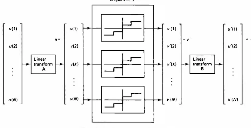
produce a (complex) vector v such that its components v(k) are mutually
uncorrelated (Fig. 11. 15). After quantizing each component v (k) independently,
the output vector v· is linearly transformed by a matrix B to yield a vector u·. The
problem is to find the optimum matrices A and B and the optimum quantizers such
that the overall average mean square distortion
l
[ N
]
1D = NE
n�l
(u(n) - u· (n))2 =NE[(u - uY (u - u")]
is minimized. The solution of this problem is summarized as follows:
(11.42)
1. For an arbitrary quantizer the optimal reconstruction matrix B is given by
498
where r is a diagonal matrix of elements "/k defined as
D.. >..k
"/k = --;->..k
>..k � E[v(k)v· *(k)],
Image Data Compression
(11 .43)
(11.44a)
(11.44b)
u =
u( l ) v( l )
v =
u(2) v(2)
Linear
v(k)
A
N quantizers
v"( l )
v"(2)
v"(k) = v
Linear transform
B
u'(l )
= u·
u"(2)
u(N) v(N) v"(N) u"(N)
Figure 11.15 One-dimensional transform coding.
2. The Lloyd-Max quantizer for each v(k) minimizes the overall mean square
error giving
r = I (11.45)
3. The optimal decorrelating matrix A is the KL transform of u, that is, the rows
of A are the orthonormalized eigenvectors of the autocovariance matrix R.
This gives
B = A-1 = A*r (11 .46)
Proofs
1. In terms of the transformed vectors v and v· , the distortion can be written as
D =
�
E{Tr[A-1 v - Bv")[A-1 v - Bv']*1}= _!_ TrN [A-1 A(A -1)*r + BA'B*r - A-1 AB*r - BA *r ( A-1)*7]
where
A � E [vv*7], A' � E[v'(v")*7], A � E[v(v')*7]
(11 .47a)
(11.47b)
(11.47c)
Since v (k), k = 0, 1 , . .. , N -1 are uncorrelated and are quantized indepen
dently, the matrices A, A', and A are diagonal with A.k > 'A.ic, and �k as their
respective diagonal elements. Minimizing D by differentiating it with respect
to B* (or B), we obtain (see Problem 2. 15)
Sec. 1 1 .4
BA" -A-1A= 0
�
B = A-1 A. (A't1 (11 .48)which gives (11.43) and
D = _!_ Tr[ A -I E[v - rv·][v - rv·]*T (A-1)*T)
N (11.49a)
2. The preceding expression for distortion can also be written in the form
N-IN-1
D = _!_
2:: 2::
l[A-1]i,k l20-� (k)>..k (11 .49b)500
N i = O k = O
where �(k) is the distortion as if v (k) had unity variance, that is
0-� (k) � E[lv (k) - "/kv· (k)l2]/>..k (11.49c)
From this it follows that 0-� (k) should be minimized for each k by the quan
tizer no matter what A is. t This means we have to minimize the mean square
error between the quantizer input v (k) and its scaled output "/k v· (k). Without
loss of generality, we can absorb 'Yk inside the quantizer and require it to be a
minimum mean square quantizer. For a given number of bits, this would be
the Lloyd-Max quantizer. Note that 'Yk becomes unity for any quantizer whose
output levels minimize the mean square quantization error regardless of its
decision levels. For the Lloyd-Max quantizer, it is not only that 'Yk equals
unity, but also its decision levels are such that the mean square quantization
error is minimum. Thus (11.45) is true and we get B = A-1. This gives
(11.50) where f(x) is the distortion-rate function of an x-bit Lloyd-Max quantizer for unity variance inputs (Table 4.4). Substituting (11.50) in (11 .49b), we obtain
D =
�
Tr[A-1 FA(A-1)*TJ,Since v equals Au, its covariance is given by the diagonal matrix
E[vv*T) � A = ARA*r
Substitution for A in (11.51) gives
D =
�
Tr[A-1 FAR](11.51)
(11 .52)
(11 .53)
where F and R do not depend on A. Minimizing D with respect to A, we obtain
(see Problem 2.15)
0 = iJD = -iJA _!_ [A-1 FARA -iy + _!_ [RA -l Ff
N N
:::} F(ARA-1) = (ARA-1)F (11.54)
Thus, F and ARA -i commute. Because F is diagonal, ARA -1 must also be
diagonal. But A�A *Tis also diagonal. Therefore, these two matrices must be
related by a diagonal matrix
G,
ast Note that 0-�(k) is independent of the transform A.
ARA *T = (ARA -1)G (11.55)
This implies AA *T = G, so the columns of A must be orthogonal. If A is
replaced by G112 A, the overall result of transform coding will remain un
changed because B = A -1 • Therefore, A can be taken as a unitary matrix,
which proves (11.46). This result and (11.52) imply that A is the KL transform
of u (see Sections 2.9 and 5.11).
Remarks
Not being a fast transform in general, the KL transform can be replaced either by a fast unitary transform, such as the cosine, sine, DFT, Hadamard, or Slant, which is not a perfect decorrelator, or by a fast decorrelating transform, which is not unitary.
In practice, the former choice gives better performance (Problem 11.9).
The foregoing result establishes the optimality of the KL transform among all decorrelating transformations. It can be shown that it is also optimal among all the unitary transforms (see Problem 11 .8) and also performs better than DPCM (which can be viewed as a nonlinar transform; Problem 11.10).
Bit Allocation and Rate-Distortion Characteristics
The transform coefficient variances are generally unequal, and therefore each requires a different number of quantizing bits. To complete the transform coder design we have to allocate a given number of total bits among all the transform coefficients so that the overall distortion is minimum. Referring to Fig. 1 1 . 15, for
any unitary transform A, arbitrary quantizers, and B = A-1 = A *T; the distortion
becomes
N- 1 N- 1
D =
� k�o
E [Jv (k) - v· (k)l2] =� k�o CJ U(nk)
(11.56)where CJ i is the variance of the transform coefficient v (k), which is allocated
nk
bits,and /(-), the quantizer distortion function, is monotone convex with f(O) = 1 and
f(oo) = 0. We are given a desired average bit rate per sample, B ; then the rate for the
A-transform coder is
(1 1.57)
The bit allocation problem is to find
nk
�
0 that minimize the distortion D, subjectto (11.57). Its solution is given by the following algorithm.
Bit Allocation Algorithm
Step 1. Define the inverse function off '(x) � df(x)ldx as h (x) �f '-1 (x), or
h (f '(x)) = x. Find 0, the root of the nonlinear equation
Sec. 1 1 .4
RA � .!. 2: h
((et
= B (1 1 .58)Nk:<YZ>O CJk
The solution may be obtained by an iterative technique such as the Newton method. The parameter
0
is a threshold that controls which transform coefficients are to be coded for transmission.Step 2 . The number of bits allocated to the kth transform coefficient are
given by
(11.59)
Note that the coefficients whose mean square value falls below 0 are not coded at
all.
Step 3. The minimum achievable distortion is then
D �
�
[,I,
rrlf(n.) + ,�<•
rrl]
(11 .60)Sometimes we specify the average distortion D = d rather than the average rate B.
In that case (11.60) is first solved for 0. Then (11.59) and (11 .58) give the bit
allocation and the minimum achievable rate. Given nk, the number of quantizer
levels can be approximated as Int[2nk]. Note that nk is not necessarily an integer.
This algorithm is also useful for calculating the rate versus distortion characteristics of a transform coder based on a given transform A and a quantizer with distortion
function f (x ).
In the special case of the Shannon quantizer, we have f(x) = 2-2x, which gives
f '(x) = - (2 loge 2)2-2x � h (x) = -! log2
N - 1
(
2)
1 I CT k
= - L max 0, 2 log29
N k �O
(11 .61)
(11.62)
(11.63)
More generally, whenf(x) is modeled by piecewise exponentials as in Table 4.4, we can similarly obtain the bit allocation formulas (32] . Equations (11.62) and (11.63)
give the rate-distortion bound for transform coding of an N x 1 Gaussian random
vector u by a unitary transform A. This means for a fixed distortion D, the rate RA
will be lower than the rate achieved by using any practical quantizer. When D is
small enough so that 0 <
0
< min k {cr U, we get 0 = D, and(11.64)
In the case of the KL transform' cr i = }\k and
n
}\k =IRI'
which givesk
For small but equal distortion levels,
RA - RKL = log2
[
c0:
cri)/IRI]
� 0where we have used (2.43) to give
N - 1 N - 1
IRI
= IARA *71 :5 k=On
[ARA *1lk, k = k=On
cr iFor PCM coding, it is equivalent to assuming A = I, so that
(11.65)
(11.66)
(11.67) where R = {r(m, n )/cr �} is the correlation matrix of u, and cr � are the variances of its
elements.
Example 11.3
The determinant of the covariance matrix R =
{p1m
-nl} of a Markov sequence of lengthN
is IR I =(1 - p2)N-
i _ This givesN - l ( 2) 1 1
DRKL = 2N log2
1 - p - 2
og2 ,(11.68)
For
N
=16
andp = 0.95,
the value of min{>..k} is0.026
(see Table5.2).
So for D =0.01,
we get RKL =
1.81
bits per sample. Rearranging(11.68)
we can write1 (1 - p2) 1 ( 2)
RKL
= 2
-2N
log21 -
P(11.69)
As
N
� oo, the rate RKL goes down to a lower bound RKL (oo) = � log2(1 - p2)/D,
and RPcM - RKL (oo) = -! log2(1 - p2) = 1.6
bits per sample. Also, as N � oo, theeigenvalues of R follow the distribution >..(w)
= (1 - p2)/(1 + p2 + 2p
cosw), whichgives min{>..k} =
(1 -:- p2)/(l + p)2 = (1 - p)/(l + p).
Forp = 0.95,
D= 0.01
we obtainRKL (oo) =
1.6
bits per sample.Integer Bit Allocation Algorithm. The number of quantizing bits nk are often
specified as integers. Then the solution of the bit allocation problem is obtained by
applying a theory of marginal analysis [6, 21], which yields the following simple
algorithm.
Step 1 .
Step 2. Start with the allocation n2
= 0, 0 :5 k s N -1. Set j = 1. ni = ni- 1 + 8(k - i), where i is any index for which
Ak � cri [f(ni- 1) -f(nt 1 + 1)]
is maximum. Ak is the reduction in distortion if the jth bit is allocated to the kth
quantizer.
Step 3. If Lk n{ ;;::: NB, stop; otherwise j � j + 1 and go to Step 2.
If ties occur for the maximizing index, the procedure is successively initiated
with the allocation n{ = nic- 1 +
8(i - k)
for each i. This algorithm simply means thatthe marginal returns
!:J,, 2 . .
!:J..k.i = CJ df(nD -f(n� + 1)],
k
= O, . . . ,N - 1,j = 1, . . . , NB (11 .70) are arranged in a decreasing order and bits are assigned one by one according to this order. For an average bit rate of B, we have to search N marginal returns NB times. This algorithm can be speeded up whenever the distortion function is of the formf(x)
= a2-b ... Then !:J..k.i = (1 - rb)CJ' i f(n{- 1), which means the quantizer having thelargest distortion, at any step j, is allocated the next bit. Thus, as we allocate a bit, we update the quantizer distortion and the step 2 of the algorithm becomes:
Then
Step 2: Find the index i such that
D; = max [CJ U(n�- 1)] is maximum k
n{ = nt 1 +
8(k
-i)D; = 2-b D;
The piecewise exponential models of Table 4.4 can be used to implement this step.
1 1 .5 TRANSFORM CODING OF IMAGES
The foregoing one-dimensional transform coding theory can be easily generalized
to two dimensions by simply mapping a given N x M image u(m, n) to a one
dimensional NM x 1 vector u. The KL transform of u would be a matrix of size
NM x NM. In practice, this transform is replaced by a separable fast transform such
as the cosine, sine, Fourier, Slant, or Hadamard; these, as we saw in chapter 5, pack
a considerable amount of the image energy in a small number of coefficients. To make transform coding practical, a given image is divided into small rectan
gular blocks, and each block is transform coded independently. For an N x M
image divided into NM!pq blocks, each of size p x q, the main storage require
ments for implementing the transform are reduced by a factor of NM lpq. The computational load is reduced by a factor of log2 MN /log2pq for a fast transform
requiring a.N log2 N operations to transform an N x 1 vector. For 512 x 512 images
divided into 16 x 16 blocks, these factors are 1024 and 2.25, respectively. Although
the operation count is not greatly reduced, the complexity of the hardware for implementing small-size transforms is reduced significantly. However, smaller block sizes yield lower compression, as shown by Fig. 11.16. Typically, a block size
of 16 x 16 is used.
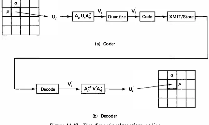
Two-Dimensional Transform Coding Algorithm. We now state a practical
transform coding algorithm for images (Fig. 11. 17).
2.5
t
2.0Qj )(
:e-�
:.a i "' 1 .5 a:
1 .0
2 X 2 4 X 4 8 X 8 1 6 X 1 6 32 X 32 64 X 64 1 28 X 1 28
81ock size
-Figure 11.16 Rate achievable by block KL transform coders for Gaussian random fields with separable covariance function, p = p2 = 0.95, at distortion D = 0.25%.
q
V;
AP U;Aq Quantize
(a) Coder
V;
Decode A;rv;A; U;
(b) Decoder
Figure 11.17 Two-dimensional transform coding.
XMIT/Store
q
1. Divide the given image. Divide the image into small rectangular blocks of size
p x q and transform each block to obtain V; , i = 0, ... , I -1 , I � NM lpq.
2. Determine the bit allocation. Calculate the transform coefficient variances <T �. /
via (5.36) or Problem 5.29b if the image covariance function is given. Alterna
tively, estimate the variances & L from the ensemble of coefficients V; (k, l),
i = 0, . .. , I -1, obtained from a given prototype image normalized to have
unity variance. From this, the <T �. 1 for the image with variance <T 2 are estimated
as cd, 1 = cr �.I CT 2. The cr L can be interpreted as the power spectral density of
the image blocks in the chosen transform domain.
The bit allocation algorithms of the previous section can be applied
after mapping CT�. / into a one-dimensional sequence. The ideal case, where
f(x) = 2-ix, yields the formulas
Alternatively, the integer bit allocation algorithm can be used. Figure 11.18
shows a typical bit allocation for 16 x 16 block coding of an image by the
cosine transform to achieve an average rate B = 1 bit per pixel.
3. Design the quantizers. For most transforms and common images (which are
nonnegative) the de coefficient v; (0, 0) is nonnegative, and the remaining
coefficients have zero mean values. The de coefficient distribution is modeled
by the Rayleigh density (see Problem 4.15). Alternatively, one-sided Gaussian
or Laplacian densities can be used. For the remaining tranform coefficients, Laplacian or Gaussian densities are used to design their quantizers. Since the transform coefficients are allocated unequal bits, we need a different quan
tizer for each value of nk, t • For example, in Fig. 11.18 the allocated bits range
from 1 to 8. Therefore, eight different quantizers are needed. To implement
these quantizers, the input sample V; (k, l) is first normalized so that it has
unity variance, that is,
506
A· (k l) � V; (k, l)
V, ' - CT k, I ' (k, l) -4' (0, 0) (11 .72)
These coefficients are quantized by an nk. 1-bit quantizer, which is designed for zero mean, unity variance inputs. Coefficients that are allocated zero bits are
j �
block cosine transform coding of images modeled by isotropic covariance function with p = 0.95. Average rate = 1 bit per
pixel.
1 0-1
not processed at all. At the decoder, which knows the bit allocation table in
advance, the unprocessed coefficients are replaced by zeros (that is, their
mean values).
4. Code the quantizer output. Code the output into code words and transmit or store.
5. Reproduce the coefficients. Assuming a noiseless channel, reproduce the coef
ficients at the decoder as
v/
(k, /) ={ov,;
(k, l)crk, i. (k, /) E I, (ll .73)otherwise
where /1 denotes the set of transmitted coefficients. The inverse trans
formation U;0 = A *Tvi· A* gives the reproduced image blocks.
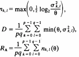
Once a bit assignment for transform coefficients has been determined, the performance of the coder can be estimated by the relations
p - l q - 1 p - l q - 1 D = plq
k
�
o 1�
0 cr�. tf(nk,1), RA = p lq k
�
o 1�
0 nk, t (11 .74)Transform Coding Performance Trade-Offs and Examples
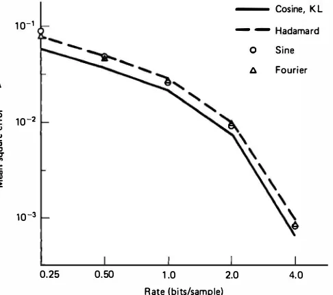
Example 11.4 Choice of transform
0.25
Figure 1 1 . 19 compares the performance of different transforms for 16 x 16 block
coding of a random field. Table 11.3 shows examples of SNR values at different rates.
The cosine transform performance is superior to the other fast transforms and is almost indistinguishable from the KL transform. Recall from Section 5.12 that the cosine transform has near-optimal performance for first-order stationary Markov sequences with p > 0.5. Considerations for the choice of other transforms are summarized in Table 11 .4.
Figure 11.19 Distortion versus rate characteristics for different transforms for a two-dimensional isotropic random field.
TABLE 1 1 .3 SNR Comparisons of Various Transform Coders for Random Fields
with Isotropic Covariance Function, p = 0.95
Block
Sine Fourier Hadamard
8 X 8 0.25 11 .74 11.66 9.08 10. 15 10.79
Note: The KL transform would be nonseparable here.
Example 11.5 Choice of block size
The effect of block size on coder performance can easily be analyzed for the case of separable covariance random fields, that is, r(m, n) = p1ml + lnl . For a block size of suitable for p = 0.95. For higher values of the correlation parameter, p, the block size
should be increased. Figure 11.20 shows some 16 x 16 block cod�d results.
Example 11.6 Choice of covariance model
The transform coefficient variances are important\for designing the quantizers. Al though the separable covariance model is convenient for analysis and design of transform coders, it is not very accurate. Figure 11.20 shows the results of 16 x 16
cosine transform coders based on the separable covariance model, the isotropic covar iance model, and the actual measured transform coefficient variances. As expected, the actual measured variances yield the best coder performance. Generally, the isotropic covariance model performs better than the separable covariance model.
Zonal Versus Threshold Coding
Examination of bit allocation patterns (Fig. 11. 18) reveals that only a small zone of
transformed image is transmitted (unless the average rate was very high). Let N1 be
the number of transmitted samples. We define a zonal mask as the array
508
m (k, !) =
{l,
k, l E /, (11 .76)0, otherwise
(a) separable, SNR' = 37.5 dB, the right side shows error images
(b) isotropic, SNR' = 37.8 dB
. i a,a
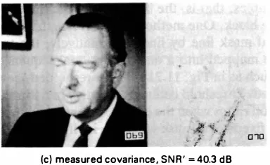
(c) measured covariance, SNR' = 40.3 dB
Figure 1 1.20 Two-dimensional 16 x 16 block cosine transform ceding at 1 bit/pixel rate using different covariance models. The right half shows error images. SNR' is defined by eq. (3. 13).
which takes the unity value in the zone of largest N1 variances of the transformed
samples. Figure ll.21a shows a typical zonal mask. If we apply a zonal mask to the transformed blocks and encode only the nonzero elements, then the method is
called zonal coding.
In threshold coding we encode the N1 coefficients of largest amplitude rather
than the N, coefficients having the largest variances, as in zonal coding. The address
set of transmitted samples is now
I/ = {k, l; lv (k, l)I > 11} (11 .77)
where 11 is a suitably chosen threshold that controls the achievable average bit rate.
For a given ensemble of images, since the transform coefficient variances are fixed,
Sec. 1 1 .5
0 0 0 0
0 0 0 0 0
(a) Zonal mask (b) Threshold mask (c) Ordering for threshold coding
Figure 11.21 Zonal and threshold masks.