isprsarchives XL 7 W4 87 2015

HYPERSPECTRAL ANALSIS OF SOIL TOTAL NITROGEN IN SUBSIDED LAND

USING THE LOCAL CORRELATION MAXIMIZATION-COMPLEMENTARY

SUPERIORITY METHOD

L.X. Lin, Y.J. Wang*, J.Y. Teng, X.X. Xi

School of Environment Science and Spatial Informatics, China University of Mining and Technology, Xuzhou 221116, China-wyj4139@cumt.edu.cn

Commission VII, WG VII/6

KEYWORDS: hyperspectral analysis, local correlation maximization-complementary superiority (LCMCS), soil total nitrogen, subsided land

ABSTRACT:

The measurement of soil total nitrogen (TN) by hyperspectral remote sensing provides an important tool for soil restoration programs in areas with subsided land caused by the extraction of natural resources. This study used the local correlation maximization-complementary superiority method (LCMCS) to establish TN prediction models by considering the relationship between spectral reflectance and TN based on spectral reflectance curves of soil samples collected from subsided land determined by synthetic aperture radar interferometry (InSAR) technology. Based on the 1655 selected effective bands of the optimal spectrum (OSP) of the first derivate differential of reciprocal logarithm ([log{1/R}]'), (correlation coefficients, P < 0.01), the optimal model of LCMCS method was obtained to determine the final model, which produced lower prediction errors (root mean square error of validation [RMSEV] = 0.89, mean relative error of validation [MREV] = 5.93%) when compared with models built by the local correlation maximization (LCM), complementary superiority (CS) and partial least squares regression (PLS) methods. The predictive effect of LCMCS model was optional in Cangzhou, Renqiu and Fengfeng District. Results indicate that the LCMCS method has great potential to monitor TN in subsided land caused by the extraction of natural resources including groundwater, oil and coal.



Corresponding author

1. INTRODUCTION

In recent years, land subsidence caused by the extraction of natural resources such as groundwater (Pacheco-Martinez et al., 2013; Bakr, 2015) oil (Moghaddam et al., 2013) and coal (Xu et al., 2014; Demirel et al., 2011) has created a severe and widespread hazard in China, resulting in new ecological and environmental issues such as soil degradation and a loss of biodiversity. As an essential element for plant growth, soil total nitrogen (TN) plays an important role in soil restoration programs. Monitoring of TN has stirred the interest of many scholars and resulted in a series of achievements recently (Endale et al., 2011;Reynolds et al., 2013); however, most approaches are based on traditional methods, which tend to be time consuming, laborious, and expensive (Chang et al., 2001). Therefore, researchers have sought real-time methods of monitoring of TN content of soils.

Hyperspectral remote sensing provides an abundance of spectral information suggesting a potential method for estimating TN (Dematte et al., 2004). Compared with traditional laboratory methods, hyperspectral techniques are more rapid, less costly, and can eliminate the need for sample preparation and chemical reagents (Chang et al., 2002; Dematte et al., 2004). Therefore, many studies have reported on various TN monitoring models (Fystro, 2002; Mutuo et al., 2006). For example, Dalal et al.

(Dalal and Henry, 1986) and Morra et al. (Morra et al., 1991) both used stepwise multiple linear regression for the rapid quantification of TN contents. Sun et al. (Sun et al., 2014) estimated TN using wavelet analysis and transformation. Zheng et al. (Zheng et al., 2008) quantified TN content through near-infrared reflectance (NIR) spectroscopy and use of a BP neural network. Partial least squares regression (PLS) has advantages in treating very large data matrices such as those typically employed with hyperspectral reflectance data; therefore, this technique has been successfully applied to spectral data for predicting soil nitrate (Ehsani et al., 1999) and organic matter content (Nocita et al., 2011; Vohland et al., 2011), and also has been employed for predicting TN (Pan et al., 2012; Kuang and Mouazen, 2013). Shi et al. (Shi et al., 2013) compared three methods for estimating TN content with visible/near-infrared reflectance (Vis/NIR) of selected coarse and heterogeneous soils, and the PLS model performed best. Chang et al. (Chang et al., 2005) integrated near-infrared reflectance spectroscopy (NIRS) and PLS to predict several soil properties including TN. In general, many studies have confirmed that PLS was one of the most efficient methods used for constructing reliable models in wide range of fields, including in the field of hyperspectral remote sensing (Nguyen and Lee, 2006).

of a neural network, have been widely used in many fields because of its usefulness with complex nonlinear problems (Sharma et al., 2015; Jang, 1993; Paiva et al., 2004; Abbasi and Abouec, 2008; Mukerji et al., 2009; Pramanik and Panda, 2009; Yan, 2010); ANFIS has also been applied to the hyperspectral assessment of soil properties (Tan et al., 2014). Although it is difficult to make full use of hyperspectral data because of the restriction on the number of input variables, ANFIS may be a promising technique in the field of hyperspectral remote sensing.

In summary, some research achievements have been accumulating with respect to estimating TN using hyperspectral remote sensing technology. Nevertheless, very little study has been undertaken in areas of subsided land where serious soil degradation is typical. In addition, almost no analysis of TN in subsided land caused by the extraction of various resources currently exists. Therefore, several issues should be considered to provide satisfactory prediction accuracy, such as whether the existing TN estimation models are suitable for used in this type of area experiencing subsidence, how to reduce noise while retaining as much useful information as possible in remotely sensed hyperspectral data, and how to realize the complementary superiority of PLS and ANFIS to further improve the accuracy of estimates of TN.

In this study, the local correlation maximization (LCM) de-noising method was used to maximize the use of TN response information and eliminate the interference of noisy data. Then based on the complementary

superiority of PLS and ANFIS to each other, the LCMCS models were built and assessed.

2. MATERIALS AND METHODS

2.1 Experimental Section

2.1.1 Sample Preparation

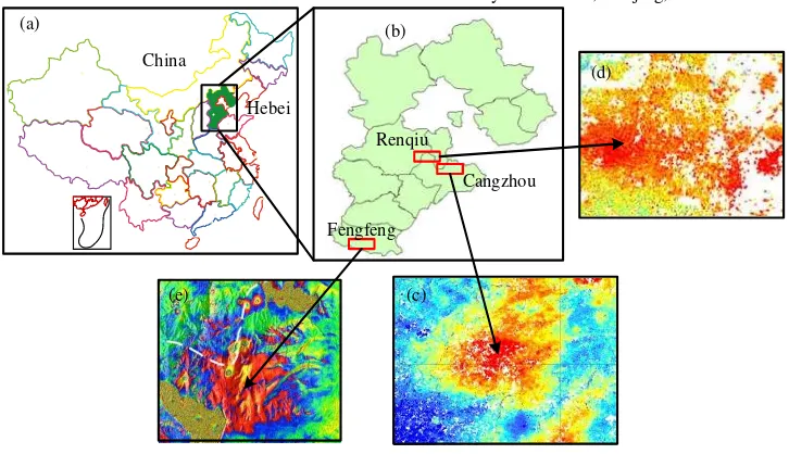
The topsoil (0–20 cm) samples analyzed in this study had been randomly collected from different soil types at 280 randomly selected sites in land that had subsided (red regions in Figure 1) of Cangzhou (Figure 1c; 38°32′N, 116°45′E), Renqiu (Figure 1d; 38°42′N, 116°7′E) and Fengfeng District (Figure 1e; 36°20′N, 114°14′E), all in Hebei Province, China. Subsidence had been caused by the excessive extraction of groundwater, oil and coal in these three areas, respectively. In this study, the subsidence deformation data of Cangzhou and Renqiu were obtained by permanently scattered interferometric synthetic aperture radar technology (Perrone et al., 2013), while data for Fengfeng District were captured by differential synthetic aperture radar interferometry technology (Chatterjee et al., 2006). All 280 soil samples were air dried, gently crushed, passed through a 2-mm sieve, and then pulverized by grinding. The samples were split into two parts with the two parts used for chemical analysis and spectral measurement, respectively. The percentage of TN in each soil sample was determined by the Institute of Soil Science, Chinese Academy of Sciences, Nanjing, China.

银川 China

Renqiu

Cangzhou

Fengfeng Hebei

(c)

(d)

(e)

(a) _(b)

Figure 1. (a) Vicinity map of Hebei Province within China; (b) Vicinity map of the Changzhou, Fengfeng, and Renqiu study sites within Hebei; Soil sample collection sites from subsided land (red regions) of Changzhou (c), Renqiu (d) and

Fengfeng (e).

2.1.2 Measurement and Data Processing

An ASD FieldSpec 3 spectroradiometer (Analytical Spectral Devices, Boulder, CO, USA) was used to measure the spectra of soil samples over wavelength ranges of 350–1000 nm and 1000–2500 nm, with increments of 1.4 nm and 2 nm, respectively. The spectral resolution at 700 nm was 3 nm; at 1400 nm and 2100 nm it was 10 nm. Each soil sample was placed in a

spectral reflectance of the soil samples was calculated, which was regarded as the original spectrum (Shi et al., 2014).

2.1.3 Spectral Transformations

Derivative processing helps to reduce the influence of low-frequency noise (Ghiyamat et al., 2013; Liaghat et al., 2014). In the reciprocal logarithm mode, spectra differences of the visible-light region can be highlighted and the influence of changes in illumination can be minimized (Wang et al., 2009). In this study, each original spectral reflectance (REF) was mathematically manipulated into the first derivative differential (FDR), reciprocal logarithm (log[1/R]) and the first derivative differential of reciprocal logarithm ([log{1/R}]').

2.1.4 Retrieval Model

As many studies have confirmed that PLS was one of the most efficient methods used in constructing reliable models in the field of hyperspectral remote sensing; therefore, this paper used PLS analysis to analyze the first issue of whether the existing TN estimation models are suitable to land that had subsided because of the excessive extraction of different resources. And LCM and CS methods were specifically aimed at second and third issues considered in this study. Finally, in order to solve all three isssues, the LCMCS method was used to retrieve the TN content. And the results were compared and evaluated.

In this study, 150 soil samples were used to construct all models (55, 50 and 45 soil samples from subsided land of Cangzhou, Renqiu and Fengfeng, respectively), In addition, in order to fully validate the prediction abilities of all model, 130 soil samples were used in verification (45, 45 and 40 soil samples from subsided land of Cangzhou, Renqiu and Fengfeng, respectively).

2.2 Theories Section

2.2.1 Local Correlation Maximization De-noising Method (LCM)

The soil spectral reflectance curves always have obvious burrs, which show that a large number of noisy data exist within the spectrum; this noise is also present in the transformed spectrum. How can noise be reduced while retaining as much useful information as possible? Based on the concept of local optimization, this study employed the LCM de-noising method to solve this difficult problem. The main steps of LCM are as follows:

(1) Decomposing the original and transformed spectrum into five layers using a wavelet denoising method that was based on the Sym8 matrix function.

(2) Calculating the correlation coefficients for the measured TN content compared with both initial (including original and transformed spectrum, the same below) and decomposed spectral reflectance (1–5 levels), in the range of 350–2500 nm.

(3) Finding the optimal decomposition level of each band, which has the maximum correlation coefficient among initial and decomposed spectra (1–5 levels) at

each wavelength; then, the corresponding correlation coefficient and decomposed band are taken as the local optimal correlation coefficient (LOCC) and optimal band (OB). After all the LOCCs and OBs are acquired, the overall LOCC and OB determined the optimal correlative curve (OCC) and the optimal spectra (OSP), respectively. Lastly, the OSP and OCC of original and transformed spectra were obtained.

2.2.2 Partial Least Square Regression Analysis (PLS)

The PLS method proposed by Gerlach, et al. (Gerlach et al., 1979) is a mainstream, linear multiple regression method that compresses spectral data by reducing the measured collinear spectral variables to a few non-correlated latent variables or factors (Geladi and Kowalski, 1986; Feret et al., 2011; Singh et al., 2013). The basic aim of PLS is to build a linear model about X (response variables matrix) and Y (predictor variables matrix). The main principle is as follows (Lin et al., 2014):

First, X and Y are decomposed into feature vectors in the forms of Equations (1) and (2):

YUQF (1)

XTPE (2)

where U and T are the score matrices, Q and P are the loading matrices, and F and E are the error matrices

(Cho et al., 2007). According to the correlation between feature vectors, a regression model is established by decomposing X and Y:

UTBEd (3)

where Ed is the random error matrix, and B is the regression coefficient matrix. Thus, if spectral vector x is known, the predicted TN

content y can be obtained ( )

yx UY BQ _. (4)

2.2.3 Adaptive Neuro-fuzzy Inference System

(ANFIS)

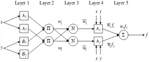
ANFIS is an adaptive neuro-fuzzy inference machine combination of fuzzy theory with neural nets (Gpyal et al., 2014). As one of the popular learning methods in neuro-fuzzy systems, a fuzzy inference system uses hybrid learning algorithms to identify the fuzzy system parameters and to teach the model (Rehman and Mohandes, 2008). Figure 2 shows the ANFIS architecture with two inputs and one output, which has five layers and two rules.

A1

Layer 2 Layer 3 Layer 4 Layer 5

x

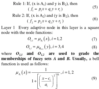
Two fuzzy if-then rules (Jang, 1992) are given as node with the node functions:

 

function is used as follows:

 

1 ₂ Layer 2 Every adaptive node in this layer multiplies the incoming signal and sends the product out; the output is determined by:

   

2,i i Ai Bi , 1, 2

O w x  y i (10)

Layer 3 Ratio of the rules for firing strength to the sum of all rule’s firing strengths is given as:

3, Layer 5 Fixed node computes the overall output as the summation of all coming signals; the output is as

To develop an ideal prediction model, this paper tried to solve several issues such as whether the existing TN estimation models were suitable for use with land that had subsided as a result of the excessive extraction of various resources such as groundwater, oil and coal, how to reduce noise while retaining as much useful information as possible, and how to realize the complementary superiority between PLS and ANFIS to further improve the estimation accuracy of models. In facing the above issues, the LCMCS method was proposed; the main steps are as follows:

(1) Spectral transforms. Spectral transforms help to reduce the influence of noise; therefore, each REF was

mathematically manipulated into FDR, log(1/R) and (log[1/R])'.

(2) LCM analysis. To maximize the use of TN response information and eliminate the interference of noisy data, OSP and OCC of the original and transformed spectrum were obtained by LCM de-noising method, which had significant correlativity with TN content.

(3) Complementary superiority. OSP and measured TN values were used in PLS analysis, and several principal components were acquired. Then these principal components and the measured TN contents were used in ANFIS analysis, and the LCMCS models were established.

(4) Model-verifying. In this study, from the 280 samples in each treatment, 150 samples were used for model calibration and the remaining 130 samples were used for model verification. Then, the best model was selected as the final model using the LCMCS method. By carefully applying spectral transforms to wavelet, correlation, PLS, and ANFIS analysis methods, the LCMCS method can effectively remove noise while preserving the detail information, taking full advantage of useful spectral information and eliminating the interference of noisy data, and the complementary superiority between PLS and ANFIS are realized.

2.2.5 Model Evaluation Standard

The stabilities and accuracies of all the models were determined by coefficient of determination (R2_{), root} mean square error of calibration (RMSEC) and mean relative error of calibration (MREC). The estimating effects were evaluated by root mean square error of validation (RMSEV) and mean relative error of validation (MREV). A good model will have a high R2, low root mean square errors (RMSEC and RMSEV), and small mean relative errors (MREC and MREV).

3. RESULTS AND DISCUSSION

3.1 Interpretation of Soil Spectral Reflectance

Figure 3. Original reflectance curve of soil samples with different TN contents.

3.2 OSP Acquirement

Each REF was mathematically manipulated into FDR, log(1/R) and (log[1/R])'. To remove the noise in the spectrum effectively, REF and the transformed spectrum were decomposed into multi-level scales using a wavelet denoising method that was based on the Sym8 matrix function. Then, correlation coefficients for the measured TN content that were compared with both the initial and the decomposed spectra (1–5 levels) were calculated. Figure 4a shows the correlation coefficients between the measured TN content and the initial FDR (data of REF,

log[1/R] and [log{1/R}]' are not shown, the same as below), and the correlation coefficients of the measured TN content with decomposed FDR (1–5 levels; Figure 4b–f). Moreover, Table 1 gives maximum values of all the correlation coefficients of initial FDR and decomposed FDR. Figure 4a–f and Table 1 demonstrate that there was a stronger correlation when the level of wavelet decomposition was 5, whose correlation coefficient reached to 0.725 (at 2316 nm). This implied that the wavelet analysis amplified some useful TN information that was previously obscured by noise.

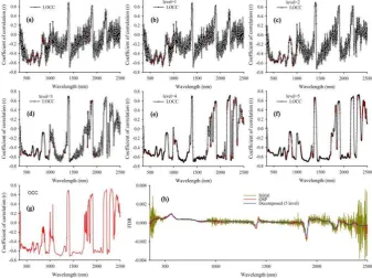
Figure 4. Wavelength dependence of coefficients of correlation between total soil nitrogen (TN) and first derivative differential of the soil spectra: initial (a); decomposed (1–5 levels) (b–f); optimal correlative curve (OCC) (g), and (h) first

TSP MPCB (nm) CC MNCB (nm) CC

FDR 1397 0.669 766 -0.672

FDR(DL=1) 1397 0.689 1419 -0.692

FDR(DL=2) 1395 0.697 1421 -0.721

FDR(DL=3) 1394 0.695 1422 -0.704

FDR(DL=4) 2205 0.714 1214 -0.715

FDR(DL=5) 2316 0.725 1223 -0.706

TSP, Types of spectral parameters; DL, Decomposition level; MPCB, Maximum positive correlation band; CC, Correlation coefficient; MNCB, Minimum negative correlation wave.

Table 1. Correlation analysis between total soil nitrogen (TN) and the first derivative differential FDR (initial and decomposed).

Then, to preserve more detail during spectra denoising, the optimal decomposition level of each band was found, which has the maximum correlation coefficient among the initial and decomposed spectra (1–5 levels) at each wavelength; the corresponding correlation coefficient and decomposed band are taken as LOCC and OB. The red points in Figure 4a–f show the LOCC and the overall

LOCC determine the OCC (Figure 4g). Figure 4h shows the initial FDR curve, decomposed FDR curve (5 level) and OSP, compared with initial FDR curve and decomposed curve (5 level); OSP can effectively remove noise while preserving the detail information simultaneously. Figure 5 shows all OCC of REF, FDR, log(1/R) and (log[1/R])'.

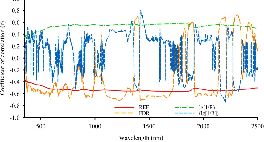
Figure 5. Optimal correlative curve of the original reflectance and its different transformation forms.

Based on Figure 5, the OCC of (log[1/R])' performed better, and the correlation coefficient was 0.797. In addition, the OCC of FDR had more bands with high correlation than OCC of (log[1/R])'; meanwhile, its maximum correlation coefficient was much higher than the OCC of REF and log(1/R). Table 2 gives their maximum correlation coefficients and number of bands at different levels of correlation. Therefore, OSP of FDR (Figure 6a) and (log[1/R])' (Figure 6b) were used to build the LCMCS model.

TSP CL NB MPCB(nm) CC MNCB(nm) CC

FDR ** 2023 2316 0.725 1421 -0.721

>0.40 1759 2316 0.725 1421 -0.721

>0.45 1654 2316 0.725 1421 -0.721

>0.50 1510 2316 0.725 1421 -0.721

>0.55 1291 2316 0.725 1421 -0.721

>0.60 949 2316 0.725 1421 -0.721

(log[1/R])' ** 1655 1422 0.797 2205 -0.739

>0.40 566 1422 0.797 2205 -0.739

>0.45 392 1422 0.797 2205 -0.739

>0.50 210 1422 0.797 2205 -0.739

>0.55 134 1422 0.797 2205 -0.739

TSP, Types of spectral parameters; CL, Correlative levels; **, at the 0.01 significance level; NB, Number of bands; MPCB, Maximum positive correlation band; CC, Correlation coefficient; MNCB, Minimum negative correlation band.

Table 2. Comparisons of the optimal correlative curve (OCC) of the first derivative differential (FDR) and the first derivative differential of reciprocal logarithm (log[1/R])'.

Spectral curves in Figure 6 shows that LCM method has strong capabilities of removing noises and preserving

detail information, which indicate that the second issue considered in this study was solved perfectly.

Figure 6. Optimal spectrum (OSP) of the first derivative differential (FDR) (a) and the first derivative differential of reciprocal logarithm (log[1/R])' (b).

3.3 Applicability of LCMCS Model

OSP and measured TN values were used in PLS analysis, and five principal components were acquired. Then these five principal components and the measured TN contents were used in ANFIS analysis, and the LCMCS models were established. Table 3 shows a comparative analysis of the performance of various models established by LCMCS method at different correlative levels of FDR (OSP) and (log[1/R])' (OSP). Based on the 1655 selected

effective bands of (log[1/R])' (OSP), whose correlation coefficients were significant (P < 0.01), the optimal model of the LCMCS method was obtained and determined to be the final model of LCMCS method, which produced more ideal results for both the calibration (R2 = 0.991, RMSEC = 0.269 and MREC = 1.446) and validation (RMSEV = 0.898 and MREV = 5.921) analyses compared with other models.

TSP CL LVs Calibration (n=150) Validation (n=130)

R2 RMSEC MREC RMSEV MREV

FDR ** 5 0.951 0.629 3.311 1.169 7.901

>0.40 5 0.946 0.667 3.818 1.095 7.901

>0.45 5 0.923 0.793 4.909 1.076 6.969

>0.50 5 0.920 0.808 5.231 1.105 6.890

>0.55 5 0.927 0.767 4.781 1.080 7.051

>0.60 5 0.917 0.821 5.168 1.184 8.068

(log[1/R])' ** 5 0.991 0.269 1.446 0.898 5.921

>0.40 5 0.939 0.704 4.220 1.529 9.613

>0.45 5 0.910 0.854 5.009 1.123 7.602

>0.50 5 0.953 0.616 3.615 1.240 8.178

>0.55 5 0.954 0.608 3.037 1.234 7.626

TSP, Types of spectral parameters; CL, Correlative levels; **, at the 0.01 significance level; LVs, Number of latent variables.

Table 3. Comparisons of the performance of models established by the local correlation maximization-complementary superiority method at different correlative levels of the first derivative differential (FDR (optimal spectrum [OSP]) and the

first derivative differential of reciprocal logarithm (log[1/R])' (OSP).

For the purpose of comparison, three issues were separately considered, and the corresponding solutions are as follows:

(1) PLS method. In PLS models, decomposed FDR (5 level) and (log[1/R])' (4 level), whose correlation coefficients reached to 0.725 and 0.797, respectively, were used in PLS analysis. Based on the 1293 selected effective bands of (log[1/R])' (5 level), whose correlation coefficients were significant (P < 0.01), the optimal model of PLS method was obtained, which was selected as the final model of the PLS method.

(2) Local correlation maximization method (LCM). Facing the second issue of how to reduce noise while retaining as much useful information as possible, OSP of FDR and (log[1/R])' were used in PLS analysis.

Based on the 1655 selected effective bands of (log[1/R])' (OSP), whose correlation coefficients significant (P < 0.01), the optimal model of the LCM method was obtained and selected as the final model of LCM method. (3) Complementary superiority method (CS). The CS model, which had the advantages of PLS and ANFIS, was aimed at addressing the third issue. The same PLS models, decomposed FDR (5 level) and (log[1/R])' (4 level) were used. Based on the 382 selected effective bands of (log[1/R])' (4 level), whose correlation coefficients were greater than 0.40, the optimal model of CS method was created and the final model of LCM method was determined.

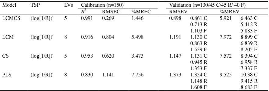
Table 4 shows results of the best model found using each method.

Model TSP LVs Calibration (n=150) Validation (n=130/45 C/45 R/ 40 F)

R2 RMSEC %MREC RMSEV %MREV

LCMCS (log[1/R])' 5 0.991 0.269 1.446 0.898 0.861 C 5.921 6.463 C

0.713 R 5.412 R

1.103 F 5.883 F LCM (log[1/R])' 8 0.916 0.804 5.498 1.191 1.130 C 7.972 8.899 C

0.863 R 6.839 R

1.529 F 8.205 F

CS (log[1/R])' 5 0.953 0.620 3.473 1.147 1.131 C 7.572 8.394 C

0.945 R 6.958 R

1.353 F 7.337 F

PLS (log[1/R])' 8 0.830 1.141 7.756 1.373 1.354 C 9.525 10.38 C

1.148 R 9.415 R

1.608 F 8.683 F

TSP, Types of spectral parameters; LVs, Number of latent variables; C, Cangzhou City; R, Renqiu City; F, Fengfeng District Table 4. Test result of the local correlation maximization-complementary superiority method (LCMCS), complementary

superiority (CS), local correlation maximization (LCM) and partial least squares regression (PLS) models for total soil nitrogen (TN) content.

The PLS model provide good results in predicting TN contents (RMSEV = 1.373, MREV = 9.525%; Table 4); this indicated that the PLS method based on spectral transforms and wavelet analysis is suitable for use with land that had subsided based on excessive extraction of different resources as discussed above. When the second issue was considered, the LCM model did perform better than the PLS model with the RMSEV of 1.191 and the MREV of 7.972%; its ability to predict was obviously enhanced at all three sites, Changzhou, Renqiu and Fengfeng. Moreover, a small improvement occurred in the CS model when compared with the LCM model, although the precision in Renqiu was reduced from 6.839% to 6.958%. The results of the LCM and CS models indicate that when second and third issues were considered, the predictive effects can be improved

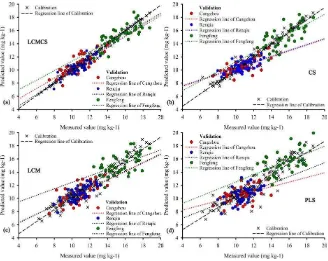
Figure 7. Comparisons of measured and predicted values by the local correlation maximization-complementary superiority method (LCMCS) (a), complementary superiority (CS) (b), local correlation maximization (LCM) (c) and partial least

squares regression (PLS) (d) methods.

4. CONCLUSIONS/OUTLOOK

By carefully applying spectral transforms as well as wavelet, correlation, PLS, and ANFIS analyses, the potential of the LCMCS method for the rapid quantification of TN was investigated. Based on the 1655 selected effective bands of (log[1/R])' (OSP), whose correlation coefficients were significant (P < 0.01), the optimal model of the LCMCS method was obtained and determined as the final model of LCMCS method. For the purpose of comparison, three issues in this study were separately considered during model establishment. The results show that all three comparative methods could quantify TN efficiently, the estimating effect of the LCM and CS models were improved more significantly than the PLS model, which respectively became the second and third issues to be taken into account, and a small amount of improvement occurred in the CS model when compared to the LCM model. However, the calculative precision of the LCMCS model improved with the consideration of the three issues; in addition, the location (Cangzhou, Renqiu or Fengfeng) did not matter and the model’s ability to estimate TN was also the most ideal. In summary, the LCMCS method has great potential for use in monitoring TN in land that had subsided because of the excessive extraction of natural resources such as groundwater, oil and coal.

ACKNOWLEDGMENTS

The National Administration of Surveying, Mapping and Geo-information of China (Grant No. 201412016), the Jiangsu Science and Technology Supporting Plan of China (Grant No. BE2012637), the Fundamental Research Funds for the Central Universities (Grant No.

KYLX_1394) and the Priority Academic Program Development of Jiangsu Higher Education Institutions supported this work.

REFERENCES

Abbasi, E., Abouec, A., 2008. Stock price forecast by using neuro-fuzzy inference system. Engineering & Technology, 46, pp. 320-323.

Bakr, M., 2015. Influence of Groundwater Management on Land Subsidence in Deltas. Water Resources Management, 29, pp. 1541-1555.

Chang, C.W., Laird, D.A., Mausbach, M.J., Hurburgh, C.R., 2001. Near-infrared reflectance spectroscopy-principal components regression analyses of soil properties. Soil Science Society of America Journal, 65, pp. 480-490.

Chang, C.W., Laird, D.A., 2002. Near-infrared reflectance spectroscopic analysis of soil C and N. Soil Science, 167, pp. 110-116.

Chang, GW, Laird, DA, Hurburgh, GR., 2005. Influence of soil moisture on near-infrared reflectance spectroscopic measurement of soil properties. Soil Science, 170, pp. 244-255.

Cho, M.A., Skidmore, A., Corsi, F., van Wieren, S.E., Sobhan, I., 2007. Estimation of green grass/herb biomass from airborne hyperspectral imagery using spectral indices and partial least squares regression. International Journal of Applied Earth Observation and Geoinformation, 9, pp. 414-424.

Dalal, R.C., Henry, R.J., 1986. Simultaneous determination of moisture, organic carbon, and total nitrogen by near infrared reflectance spectrophotometry1. Soil Science Society of America Journal, 50, pp. 120-123. multi-temporal high-resolution satellite images. International Journal of Mining Reclamation and Environment, 25, pp. 342-349.

Ehsani, M.R., Upadhyaya, S.K., Slaughter, D., 1999. A NIR technique for rapid determination of soil mineral nitrogen. Precision Agriculture, 1, pp. 217-234.

Endale, D.M., Fisher, D.S., Owens, L.B., Jenkins, M.B., Schomberg, H.H., Tebes-Stevens, C.L., Bonta, J.V., 2011. Runoff Water Quality during Drought in a Zero-Order Georgia Piedmont Pasture: Nitrogen and Total Organic Carbon. Journal of Environmental Quality, 40, pp. 969-979.

Farifteh, J., van der Meer, F., van der Meijde, M., Atzberger, C., 2008. Spectral characteristics of salt-affected soils: a laboratory experiment. Geoderma, 145, pp. 196-206.

Feret, J.B., Francois, C., Gitelson, A., Asner, G.P., Barry, K.M., Panigada, C., Richardson, A.D., Jacquemoud, S., 2011. Optimizing spectral indices and chemometric analysis of leaf chemical properties using radiative transfer modelling. Remote Sensing of Environment, 115, pp. 2742-2750.

Fystro, G., 2002. The prediction of C and N content and their potential mineralisation in heterogeneous soil samples using Vis-NIR spectroscopy and comparative methods. Plant and Soil, 246, pp. 139-149.

Geladi, P., Kowalski, B.R., 1986. Partial least-squares regression: atutorial. Anal. Analytica Chemica Acta, 185, pp. 1-17.

Gerlach, R.W., Kowalski, B.R., Wold, H.O.A., 1979. Partial least-squares path modeling with latent-variables. Analytica Chimica Acta, 3, pp. 417-421.

Ghiyamat, A., Shafri, H.Z.M., Mandiraji, G.A., Shariff, A.R.M., Mansor, S., 2013. Hyperspectral discrimination of tree species with different classifications using single- and multiple-endmember. International Journal

of Applied Earth Observation and Geoinformation, 23, pp. 177-191.

Goyal, M.K., Bharti, B., Quilty, J., Adamowski, J., Pandey, A., 2014. Modeling of daily pan evaporation in sub tropical climates using ANN, LS-SVR, Fuzzy Logic, and ANFIS. Expert Systems with Applications, 41, pp. 5267-5276.

Jang, J.S.R., 1993. ANFIS: Adaptive-network-based fuzzy inference system. IEEE Transactions on Systems, Man, and Cybernetics, part B-cybernetics, 23, pp. 665-685.

Jang, J. S. R., 1992. Self-learning fuzzy controllers based on temporal backpropagation. IEEE Transactions on Neural Networks, 3, pp. 714-723.

Kuang, B.Y.; Mouazen, A.M., 2013. Non-biased prediction of soil organic carbon and total nitrogen with vis-NIR spectroscopy, as affected by soil moisture content and texture. Biosystems Engineering, 114, pp. 249-258.

Liaghat, S.; Ehsani, R.; Mansor, S.; Shafri, H.Z.M.; Meon, S.; Sankaran, S.; Azam, S.H.M.N., 2014. Early detection of basal stem rot disease (Ganoderma) in oil palms based on hyperspectral reflectance data using pattern recognition algorithms. International Journal of Remote Sensing, 35, pp. 3427-3439.

Lin, L.X., Wang, Y.J., Xiong, J.B., 2014. Hyperspectral extraction of soil available nitrogen in nan mountain coal waste scenic spot of Jinhuagong mine based on Enter-PLSR. Spectroscopy and Spectral Analysis, 34, pp. 1656-1659. near-infrared reflectance spectroscopy. Soil Science Society of America Journal, 55, pp. 288-291.

Mukerji, A., Chatterjee, C., & Raghuwanshi, N.S., 2009. Flood forecasting using ANN, Neuro-Fuzzy, and Neuro-GA models. Journal of Hydrologic Engineering, 14, pp. 647.

Mutuo, P.K., Shepherd, K.D., Albrecht, A., Cadisch, G., 2006. Prediction of carbon mineralization rates from different soil physical fractions using diffuse reflectance spectroscopy. Soil Biology & Biochemistry, 38, pp. 1658-1664.

Nguyen, H.T., Lee, B.W., 2006. Assessment of rice leaf growth and nitrogen status by hyperspectral canopy reflectance and partial least square regression. European Journal of Agronomy, 24, pp. 349-356.

and topsoil organic carbon content through the use oflaboratory and field spectroscopy in the Albany Thicket Biome of Eastern CapeProvince of South Africa. Geoderma, 167-68, pp. 295-302.

Pacheco-Martinez, J., Hernandez-Marin, M., Burbey, T.J., Gonzalez-Cervantes, N., Ortiz-Lozano, J.A., Zermeno-De-Leon, M.E., Solis-Pinto, A, 2013. Land subsidence and ground failure associated to groundwater exploitation in the Aguascalientes Valley, Mexico. Engineering Geology, 164, pp. 172-186.

Paiva, R.P, Dourado, A., Duarte, B., 2004. Quality prediction in pulp bleaching: Application of a neuro-fuzzy system. Control Engineering Practice, 12, pp. 587-594.

Pan, T., Wu, Z.T., Chen, H.Z., 2012. Waveband Optimization for Near-Infrared Spectroscopic Analysis of Total Nitrogen in Soil. Chinese Journal of Analytical Chemistry, 40, pp. 920-924.

Perrone, G., Morelli, M., Piana, F., Fioraso, G., Nicolo, G., Mallen, L., Cadoppi, P., Balestro, G., Tallone, S., 2013. Current tectonic activity and differential uplift along the Cottian Alps/Po Plain boundary (NW Italy) as derived by PS-InSAR data. Journal of Geodynamics, 66, pp. 65-78.

Pramanik, N., Panda, R.K., 2009. Application of neural network and adaptive neuro-fuzzy inference systems for river flow prediction. Hydrological Sciences Journal, 54, pp. 247-260.

Rehman, S., Mohandes, M., 2008. Artificial neural network estimation of global solar radiation using air temperature and relative humidity. Energy Policy, 36, pp. 571-576.

Reynolds, B., Chamberlain, P.M., Poskitt, J., Woods, C., Scott, W.A., Rowe, E.C., Robinson, D.A., Frogbrook, Z.L., Keith, A.M., Henrys, P.A., 2013. Countryside Survey: National "Soil Change" 1978-2007 for Topsoils in Great Britain-Acidity, Carbon, and Total Nitrogen Status. Vadose Zone Journal, 12.

Sharma, S., Srivastava, P., Fang, X., Kalin, L., 2015. Performance comparison of Adoptive Neuro Fuzzy Inference System (ANFIS) with Loading Simulation Program C++ (LSPC) model for streamflow simulation in El Nino Southern Oscillation (ENSO)-affected watershed. Expert Systems with Applications, 42, pp. 2213-2223.

Shi, T.Z., Cui, L.J., Wang, J.J., Fei, T., Chen, Y.Y., Wu, G.F., 2013. Comparison of multivariate methods for estimating soil total nitrogen with visible/near-infrared spectroscopy. Plant and Soil, 366, pp. 363-375.

Shi, T.Z., Liu, H.Z., Wang, J.J., Chen, Y.Y., Fei, T., Wu, G.F., 2014. Monitoring arsenic contamination in agricultural soils with reflectance spectroscopy of rice plants. Environmental Science & Technology, 48, pp. 6264-6272.

Singh, A., Jakubowski, A.R., Chidister, I., Townsend, P.A., 2013. A MODIS approach to predicting stream water quality in Wisconsin. Remote Sensing of Environment, 128, pp. 74-86.

Sun, Z.G., Zhang, Y., Li, J.L., Zhou, W., 2014. Spectroscopic Determination of Soil Organic Carbon and Total Nitrogen Content in Pasture Soils. Communications in Soil Science and Plant Analysis, 45, pp. 1037-1048.

Tan, K., Ye, Y.Y., Cao, Q., Du, P.J., Dong, J.H., 2014Estimation of arsenic contamination in reclaimed agricultural soils using reflectance spectroscopy and ANFIS model. IEEE Journal of Selected Topics in Applied Earth Observations and Remote Sensing, 7, pp. 2540-2546.

Vohland, M.; Besold, J.; Hill, J.; Fründ, H.C., 2011. Comparing different multivariate calibration methods for the determination of soil organic carbon pools with visible to near infrared spectroscopy. Geoderma, 166, pp. 168-205.

Wang, Y., Wang, F.M., Huang, J.F., Wang, X.Z., Liu, Z.Y., 2009. Validation of artificial neural network techniques in the estimation of nitrogen concentration in rape using canopy hyperspectral reflectance data. International Journal of Remote Sensing, 30, pp. 4493-4505.

Xu, H.F., Liu, B., Fang, Z.G., 2014. New grey prediction model and its application in forecasting land subsidence in coal mine. Natural Hazards, 71, pp. 1181-1194.

Yan, H., Zou, Z., Wang, H., 2010. Adaptive neuro fuzzy inference system for classification of water quality status. Journal of Environmental Sciences, 22, pp. 1891-1896.