Ruin theory with risk proportional to the free reserve and securitization
Thomas Siegl
a,∗, Robert F. Tichy
baArthur Andersen, Risikomanagement Beratung, Mergenthalerallee 10-12, D-65760 Eschborn, Germany bInstitut für Mathematik, TU-Graz, Steyrergasse 30/II, A-8010 Graz, Austria
Received January 1999; received in revised form August 1999
Abstract
A model is proposed for addressing investment risk of the free reserve, in the form of credit or currency risk. This risk is expressed by a constant factorαthat represents the recovery rate of a bond or a devaluation factor. Securitization (e.g. with a CAT-bond like product) yields a constant amountKupon such an event. The model equation is an integro-differential equation with deviating arguments. We compute the analytical solution for the probability of survival and also show results of simulations using quasi-Monte Carlo methods. ©2000 Published by Elsevier Science B.V. All rights reserved.
MSC:62P05; 34K10
Keywords:Ruin theory; Credit risk; Currency risk; Securitization; Deviating arguments; Quasi-Monte Carlo method
1. Introduction
We extend the classical ruin model with the two main components of premium income and claims payment. The third component reflects a risk proportional to the free reserve such as a currency devaluation or credit event. In the later case we assume that the free reservexis invested in bonds with credit risk. Upon a credit event the value of the free reserve drops according to the recovery rateαfromx toαx. Then the free reserve is reinvested in bonds with similar risk.
Another application lies in modeling currency devaluation. We assume that the free reservexAof the insurance is invested in currency A and that claims and premiums are paid in currency B. Letxdenote the equivalent toxA in currency B. If currency A is devaluated with respect to currency B, the value of the free reservexA(with respect to the ability to pay claims) changes fromxin currency B toαxin currency B, orx→αxfor short.
Furthermore, we assume that the insurer will hedge against these events by e.g. a securitization bond where the notional is at risk. We model this hedge by a constant paymentK(the bond notional) that is added to the free reserve immediately after the eventx → αx+K. The premium for this embedded option is paid for by a continuous payment of a partcˆof the total premium incomec˜in the form of a spread over the applicable interest rate (a larger
∗Corresponding author.
regular coupon). The bond is re-emitted after the event. The proposed model may help in choosing the optimal terms of such a risk exchange.
In the following we will present the model for arbitrary claim size distributionsF and prove existence and uniqueness for the general case, while an analytic solution is found for the special caseF (y) = 1−exp(−y). Furthermore, we compare the performance of hybrid and pseudo-Monte Carlo sequences for this case. We will show that a significant improvement by a factor of 2–3 is possible as far as the required sample size for a given error is concerned.
2. Model with upper barrier
We assume that premiums are paid at a constant rate of c˜ = ˆc+c (c > 0)per unit time, that the claim number follows a Poisson processNλ(t )with parameterλ >0, and that the individual i.i.d. claimsYi ≥ 0 have
distributionF (y)with expected valueµ < ∞. Furthermore, the devaluations are rare events, and therefore the number of devaluations also follows a Poisson processNγ(t )with parameterγ >0. Upon devaluation, the reserve is multiplied by the factor 0< α <1. In this case, the embedded option pays an amount ofK >0(x→αx+K). It is financed by the continuous payment ofcˆ. At the timet (n)of thenth devaluation, the free reservexchanges to
αx+Kyielding the stochastic process of the free reserveRt at timet:
Rt =R0+ct−
Nλ(t ) X
n=1
Yn−
Nγ(t )
X
n=1
((1−α)Rt (n)−K).
If the reserveRt drops below 0, we say ruin has occurred. The infinite time survival probability is defined for the initial free reservex =R0by
U (x)=P
inf
t≥0Rt ≥0
.
However, for 0< α <1 we can always find a capital levelxsuch that the expected capital gain per unit time which is approximately
c−λµ−γ ((1−α)x−K) <−C, forC∈R+
is less than any arbitrary constant. Thus, without further restrictions, the infinite time ruin probability9(x) =
1−U (x)is 1. Therefore, we introduce an absorbing horizontal barrier atxmax. If the process reaches the barrier, it is absorbed and the company has survived. This corresponds to the situation where the company will then decide to pursue other forms of investment or securitization.
By including a barrier, the process stops in finite time with probability 1. However, the restriction by the upper barrier also forces us to restrict our choice ofK for the solution method we are going to present now. We will formulate the model equation as an integro-differential equation with deviating arguments. When we allowαx+K
to exceedxmaxwe would obtain a retarded integro-differential equation. The difficulties inherent in solving this type of equation can be shown for the special case whereλ=0. Then the model equation becomes (through the standard use of the law of total probability) a retarded differential equation:
cU′(x)−γ U (x)+γ U (αx+K) = 0,
∀x ≥xmax: U (x) = 1.
While the solution is readily seen for this boundary type (the solution isU (x) ≡1) finding a solution for other boundary conditions becomes quite a challenge. As an example we consider a boundary on [xmax,∞)defined by
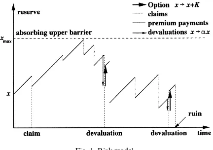
Fig. 1. Risk model.
we will just show the solution forα=2 andK=0 which corresponds to the case presented later where we allow
α >1. We find forxmax/2≤x < xmax:
U (x)=expγ
c(x−xmax)
,
and forxmax/4≤x < xmax/2:
U (x)=expγ
c(2x−xmax)
+1+exp−γ xmax 2c
expγ
c
x−xmax
2
,
which can be continued ad infinitum with increasingly complex piecewise defined functions. This solution does not even fit our model asλ=0 and should just serve as a demonstration of the difficulties encountered when we leave out the condition that after devaluation the capital may not exceedxmax. Thus, we restrict ourselves to the natural conditionαx+K ≤xmaxforx ∈ [0, xmax]. This is equivalent toK ≤ (1−α)xmax. This means that the securitization payout must not exceed the maximal loss by devaluation. Thus, there is no speculative element in the securitization, but only the hedging element. The situation is depicted in Fig. 1.
For further reference concerning models with absorbing horizontal barrier see Dickson (1991), and Dickson and Gray (1984), and for general linear barriers Gerber (1981), and Siegl and Tichy (1996). The known solutions of the problems with general linear barriers are given by infinite series in terms associated with the case without barrier. We expect the solution of our problem with a general linear barrier to be substantially more difficult, as the simpler case of a horizontal barrier leads to an infinite series already.
The law of total probability in an infinitesimal time intervalτ yields the model equation for the probability of survivalU (x)depending on the initial surplusx
U (x)=(1−λτ−γ τ )U (x+cτ )+λτ
Z x
0
U (x−y)dF (y)+γ τ U (αx+K)+O(τ2),
with the boundary condition
U (xmax)=1, (1)
at the horizontal absorbing upper barrierxmax. Note that we have a one-point boundary in contrast to the example presented before, where we hadα > 1. We can transform the model equation by a Taylor expansion and some simplifications to the integro-differential equation with deviating argument:
cU′(x)−(λ+γ )U (x)+λ
Z x
0
3. Analytic solution
The analytic solution will solve the case whereF (y)=1−exp(−βy)is the exponential distribution. Without loss of generality we can restrict ourselves to the parameter of the exponential distributionβ =1. As we will solve the equation by a series type solution we will group together certain parts of the equation and try to eliminate each group. This solution procedure is very convenient for this type of problem, but looks unusual for everyone trying to solve the equation as a whole.
Eq. (2) is an integro-differential equation with deviating argument. For the theory of differential equations with deviating argument see, e.g. El’sgol’ts and Norkin (1973). One way to obtain a solution for (2) is to convert this equation by differentiating it with respect toxand solving the resulting differential equation with deviating argument. However, there is no obvious gain by this, and thus we will solve the equation directly by using a solution of the form: forget Eq. (5) for a moment,
X coefficient of exp(Ri,jx)by settingR1,0andR2,0equal to the two solutions of the quadratic equation resulting from Eq. (4):
cR−(λ+γ )+λ 1
R+1 =0. (7)
Next, we will eliminate the terms resulting from (6) by a restriction to the coefficients
X
(i,j )∈I Ai,j Ri,j +1 =
0. (8)
What remains is to eliminate the terms that were newly introduced byU1,0 andU2,0 in the part with deviating argument (Eq. (5)). To do so let us rewrite Eqs. (4)+(5)+(6) once more, withRi,j = αRi,j−1. Furthermore, in writing down the equation we rewrite the indices using exp(Ri,jx)=exp(αRi,j−1x),
+ X
and change the summation index to avoid references to the indexj−1. Finally we insert exp(Ri,jx)=exp(αRi,j−1x) and obtain
The terms in Eq. (12) were eliminated by restriction (Eq. (7)) to the exponentsRi,j=0, and Eq. (15) was already
eliminated by restriction (Eq. (8)) to the coefficientsAi,j. The remaining terms in the equation can be eliminated by
a further restriction to the coefficientsAi,j. This can be achieved by a recursion of the following type. We assume Ai,j−1andRi,j−1are known and set,
In other words, we introduce a new remainder for every part of Eq. (5) that has not been canceled out already. Of course this will generate further terms that have to be canceled out later. As long as this remainder converges to 0 forj → ∞the series will solve the equation at the limit. Asα <1, we haveRi,j →0 (i=1,2) forj → ∞, and
thus we require that the coefficients converge as well:
Table 1
Parameters for the numerical experiments
Parameter c λ γ α xmax K
Value 11/10 1 1/10 9/10 10 1
Due to Eq. (17) and asRi,j → 0 forj → ∞, the maximum norm of the remaining defect goes to 0 asj → ∞.
Finally, we want to fit the solution to the boundary value and get the restriction
U (xmax)=1. (18)
We have three arbitrary coefficientsA0,0, A1,0andA2,0and three equations (18), (17) and (8). Thus, our solution is the only solution of the form (3). What remains is to show that the solution is unique.
The theory of differential equations with deviating arguments gives us uniqueness of the solution under the condition that the corresponding integral operator is contracting. We have chosen to prove existence and uniqueness in this way as the integral operator for Eq. (2) is of interest itself for numerical simulation.
The operator is defined by the integral equationU=I(U ), where we defineIas the expectation over time (over all events at timet, claims of sizeyand devaluations) of the expected probability of survival in each case.
I(U )(x)=
whereT =x−xmax/cis the remaining time until the barrier is hit and the additive term corresponds to the case where the barrier is reached before an event occurs. We prove that the operator is strictly contracting by using the maximum norm of the difference of two solutionsUandV
kI(U )−I(V )k∞= max
where1 =1−exp(−(λ+γ )xmax/c) <1. Therefore, we have proved contraction with an explicit contraction constant1. Depending on the given cumulative distribution functionF the contraction constant can in general be improved. In our analytic solution, we have the exponential distribution with parameter 1. This leads to a maximal contraction constant of≈0.991 for the parameters in Table 1.
Furthermore, due to the additive term exp(−(λ+γ )T ), we cannot have the trivial solutionU ≡ 0 ifxmaxis finite. By using Banach’s fixed point theorem onL∞(R+)we have proved that the solution of Eq. (3) is the only measurable bounded solution of Eq. (2) with Eq. (1).
4. Model with random time horizon
of the situation. His reserve will appreciate in value by a factorα >1. Another interpretation for such a case would be that the insurer has invested the reserve in securities which pay dividends or interest non-deterministically.
We are interested in a model where this possibility can be incorporated without sacrificing an analytical solution. To allow a solution also for the case α > 1 we drop the upper barrier from our model (also because of the mathematical intractability mentioned before), and replace the boundary condition by
lim
x→∞U (x)=1, (20)
but we can keep the additive termK ≥0 that is added upon an appreciation/devaluation event. So far, the model equation has not changed safe for the support ofU, which is now [0,∞) and the boundary condition (20). However, for the case without upper bound we do not have strict contraction of the associated integral operator on the interval
x ∈ [0,∞) and thus the approach used before for proving existence and uniqueness does not hold anymore. Moreover, for numerical simulation it is very convenient that the process stops in finite time with probability 1.
Thus, we introduce a modification to the previous situation. We consider a modification of the time horizon to a random variable with distributionG(T ). This can be interpreted as the case where the insurer stops the business after a random time. The company may then change its investment or securitization methodology. Furthermore, we assume that the company has survived in this case. This yields the model equation after similar steps as before
U (x)=
In the following we will consider the special case whereG(T )is the exponential distribution with parameterη >0:
cUx(x)−(λ+γ +η)U (x)+λ
Z x
0
U (x−y)dF (y)+γ U (αx+K)+η=0. (21)
Note that the remaining requirements for the solution (λ >0, γ >0, c >0, positive claims,µ < ∞) still hold, and that we do not need further restrictions to obtain Eq. (20) as the process stops in finite time with probability 1. Thus we can relaxαtoα >0.
5. Analytic solution
We can solve the equation by the above mentioned steps with some modifications. As the solution must stay bounded forx → ∞, no strictly positive exponents can occur in the solution
U (x)= X to the solution presented before. Inserting this into the model equation (21) gives the similar result
as before and forget Eq. (20) for the moment and concentrate on(i, j )=(1,0)giving us the restriction
cR−(λ+γ+η)+λ 1
R+1 =0, (26)
as before. We use the unique strictly negative solution asR=R1,0. Such a solution must exist and be unique which we immediately see from the canonical form of Eq. (26)
R2−c+λ+γ+η
c R−
γ +η
c =0,
and by observing thatR1,0R2,0= −(γ+η)/c <0. Next, we will eliminate the terms resulting from Eq. (25) by the restriction (Eq. (8)) to the coefficients. With this setting, the coefficientA1,0is no longer arbitrary. What remains is to eliminate the terms that are newly introduced byU1,0using a recursion as shown before. We assumeA1,j−1and
R1,j−1are known and set
In other words, we introduce for every term that has a remainder in Eq. (24) a new term that eliminates this “defect”, but introduces a new remainder. Forj → ∞, we haveRi,j → −∞fori=1,2, and we require
A1,j =0 forj → ∞, (28)
which, however, always fulfilled. In the first case we haveα >1, and easily obtain
j
and thusAi,j converges to 0. Therefore, the maximum norm of the remainder goes to 0 asj → ∞.
Again the theory of differential equations with deviating arguments gives us uniqueness of the solution under the condition that the corresponding integral operator is contracting.
This operator is strictly contracting as we get for the maximum norm of the difference of two solutionsUandV
kI(U )−I(V )k∞= max
0≤x<∞|I(U )(x)−I(V )(x)|,
by the linearity ofIthe relation
kI(U )−I(V )k∞
where1=(λ+γ )/(λ+γ+η) <1. Therefore, we have proved contraction with an explicit contraction constant.
6. Numerical solution
We consider the case with a finite upper barrier andα <1 to be the most interesting case in applications. Therefore, we will show some methods to solve this model with stochastic simulation. While the exponential distribution is very convenient for analytical arguments, it can seldom be justified in practice. However, when we develop numerical methods, we often want such a benchmark model to test the accuracy and speed of the solution. The idea is, that similar problems will have a comparable behavior.
6.1. Evaluation of the analytical solution
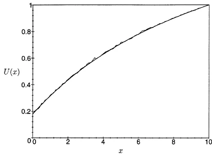
We used the parameters in Table 1 for the numerical experiments. The series in Eq. (3) was computed by truncating the series at a given indexJ =80. We have computed the free coefficients under the restrictions Eqs. (8), (17) and (18). Furthermore, we have replaced the limit in Eq. (17) by the finite truncation pointJ. The symbolic computation packageMAPLEwas used to evaluate the function. Due to the comparatively simple operations needed to solve our problem, and the fact that convergence is very fast forα≪1 the analytic solution was much faster than any simulation for comparable accuracy.
6.2. Discussion of the dependency on the parameters
Based on the parameters in Table 1 we have plotted the probability of survival atx˜=xmax/2 in Fig. 2. We have assumed that we can buy a unit of securitization payout at the cost of a continuous payment ofγ. It can be seen that the optimal securitization size isK≈0.5 withc≈1.15.
From the definition of the process we can easily see that the probability of survival at a given initial capitalxis an increasing function ofKandc. Furthermore, we obtain thatUx˜(c, K)is a concave function ofcandK. Thus,
if we finance a securitization of sizeKby a continuous payment proportional toK, we obtain a concave function ofK. Therefore, we have shown thatUx˜(c˜−γ K, K), which is depicted in Fig. 2, is a concave function ofK.
Furthermore, we can easily see thatUx˜ is a decreasing function ofxmax,λandγ, and an increasing function ofα.
6.3. Stochastic simulation
Fig. 2. Comparison of different securitization sizesKwherec= ˜c−γ K.
Fig. 3. Comparison of analytical and numerical solution. of Afflerbach (1990) based on the recursion
xi =532 393xi−1+1 (mod 268 435 456) (30) withx0 =12 785. Here, we want to note that one can find a large number of alternative efficient pseudo-random number generators which could be used instead of the Afflerbach sequence (see e.g. Fishman, 1990). Our choice is motivated by our previous experience regarding applications of the sequence in similar problems. The sequence is also used in the hybrid method presented later.
The integral operator can also be used to obtain a numerical solution for our problem by means of a simulation. We employ a hybrid Monte Carlo method that makes use of a low discrepancy sequence.
6.4. Quasi-Monte Carlo sequences
equations by simulation. One of the central definitions in this area is the discrepancy which is defined as the maximal difference between the empirical and the theoretical distribution function. We restrict ourselves to the uniform distribution.
where #{n:Bn}denotes the number ofnsatisfying conditionBncomponentwise.
Traditional Monte Carlo integration does not give an exact error bound. However, we can obtain a bound on the probable error by the Chebyshev inequality (Kalos, 1986)
P
where Var[f (x)] is the variance off (ξ ). By selecting a suitableε, we obtain that the probable error is proportional to 1/√N, which is independent ofs. This is optimal for large dimensions(s >20)and reasonableN because for large dimensions(s >20)the error bounds for quasi-Monte Carlo integration are next to useless. A deterministic error bound for such integrals is given by the Koksma–Hlawka inequality
whereV (f )is the total variation off in the sense of Hardy and Krause. For special sequences, which we will discuss next, the discrepancy satisfies
D∗N(ξ )≤Cs
(logN )s
N , (31)
with an explicitly computable constantCs (Niederreiter, 1992). The bounds for the constant are usually pessimistic and often the actual error made by quasi-Monte Carlo integration is much lower than the error bound (Caflisch, 1998). This has been observed in many applications ranging from the pricing of mortage backed securities (Papageorgiou and Traub, 1996; Paskov, 1994; Paskov and Traub, 1995) to the pricing of options (Joy et al., 1996). These recent results have one observation in common: certain quasi-Monte Carlo sequences have been shown to be superior to pseudo-Monte Carlo sequences even in large dimensions, although the error bounds for the quasi-Monte Carlo methods are worse.
Sequences that satisfy (31) are often called low-discrepancy sequences as they have the currently best asymptotic discrepancy estimates asN → ∞. Note however, that the constantCscan be influenced by the construction of the
quasi-Monte Carlo sequence.
• The constantCs for the Halton (1960) sequence tends to infinity super-exponentially for s→ ∞. This sequence
is defined as a sequence of vectors based on the digit representation ofnin basepi
ξn=(bp1(n), bp2(n), . . . , bps(n)),
wherepi is theith prime number andbp(n)is the digit reversal function for basepgiven by
bp(n)=
where thenkare integers. It is also possible to use arbitrary pairwise-coprime base numbers, but the error estimate
• The first improvement of this situation is given by the Sobol’ (1967, 1976) sequence. WhileCs still tends to infinity super-exponentially (Morokoff, 1994) the constant is much lower than that of the Halton sequence. The general definition of the Sobol’ sequence would be beyond the scope of this paper, thus we only present an elegant definition that can be found in Beck and Chen (1987) for a Sobol type sequence{(x1, y1), (x2, y2), . . .}
in dimension 2, whereaν is the binary representation ofn
n=P∞
ν=1aν2ν−1, (bν)=M(aν) (mod 2), xn=P∞ν=1aν2−ν, yn=P∞ν=1bν2−ν.
Here the matrixMi,j = i−1
j −1 !
(mod 2)consists of the binomial coefficients in the finite fieldF2.
• The Faure (1981, 1982) sequence was the first low discrepancy sequence for which the constantCs does not
grow, but tends to zero ass→ ∞.
• Further classes of low-discrepancy sequences are due to Niederreiter (1987). Among them, the Niederreiter sequence with base 2 is best suited for computation as the arithmetic can be performed modulo 2.
The Sobol’, Faure, and Niederreiter sequences are examples of so-called(t, m, s)-nets or nets for short. These nets are based on theb-adic representation of vectors in thes≥1 dimensional unit cube. Instead of optimizing the discrepancy itself, an easier task is set: to control the discrepancy over a specified set of rectanglesJ. Let #(J;N )
denote the number ofn, 1+ ≤n≤Nwithxn∈J, J ∈J, and Vol(J )the volume ofJ. Now, the idea is that we try
to obtain a low discrepancy, not for arbitrary intervals, but for a family of intervals that is convenient for mathematical analysis, such as the family ofelementary intervals in baseb. They have the formJ =Qs
i=1[aib−di, (ai+1)b−di),
with integersdi ≥0 and integers 0≤ai < bdi for 1≤i≤s.
The next idea is to look at the discrepancy ofs-dimensional intervals, not at an arbitrary length of the sequence, but rather at a powermof the baseb. We say that a point setPwith card(P)=bmis a(t, m, s)-net, if #(J;bm)=bt
for every elementary intervalJwith Vol(J )=bt−m. The parametertis a quality parameter. Ift=0, then we have minimal discrepancy of the point setP with respect to the family of elementary intervals. Based on this definition we now consider sequences.
Definition 1 ((t, s)-sequence)). Let t ≥ 0 be an integer. A sequence ξ1, ξ2, . . . of points in Is is called a
(t, s)-sequence in baseb, if for all integersk ≥ 0 andm > t the point set consisting of the ξn with kbm < n≤(k+1)bmis a(t, m, s)-net in baseb.
The theory of(t, s)-sequences is given in detail by Niederreiter (1992) and Drmota and Tichy (1997). The Sobol’ sequence is a(t, s)-sequence in base 2 with valuestthat depend ons. The Faure sequence is a(0, s)-sequence in baseps, whereps is the smallest prime number >s. The Niederreiter sequences yield(t, s)-sequences in arbitrary
base; among them there are(0, s)-sequences in prime power basesb≥s.
6.5. Numerical simulation of the integral equation
In the simulation of the integral equation we use hybrid Monte Carlo sequences for the generation of uniformly distributed sequences. The Faure (1982), Halton (1960) and Niederreiter (1987) in base 2, and Sobol’ (1976) sequences are used for the initial 48 dimensions. The pseudo-random sequence of Afflerbach (1990) is used for the remaining dimensionss≤3000.
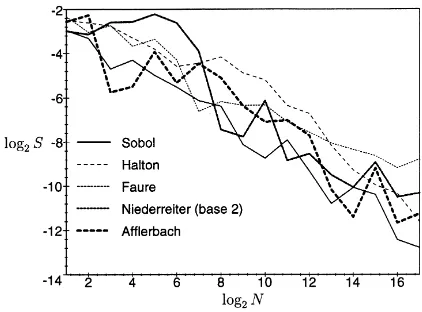
Fig. 4. Mean square error for hybrid (dim 48) and pseudo-Monte Carlo.
Fig. 5. Regression analysis of the mean square error.
algorithm, whereExp(·|z)denotes a random variable cut off atz, andMgives the recursion depth (M=1000 in our example).
Solution of the integral equation: ComputeU˜ =N1PN
n=1R(M, x0) FunctionR(m, x):
Ifm=0: Return(0);
Generatet∼Exp(λ+γ|xmax−x
c )
GenerateB∼Bernoulli(λ+λγ)
IfB=
(
1 : Generatey ∼Exp(1|x+ct )
0 : y=(1−α)(x+ct )+K
Return(1 λ+γ
−Be−x−ct)(1−e−(λ+γ )T)R(m−1, x+ct−y)+e−
(λ+γ )T
End Function
In the following experiments we compare the simulation results of different hybrid sequences with the result of the exact solution that is computed according to Section 6.1. As the initial part of the hybrid sequence is always the same due to the construction of the quasi-Monte Carlo sequence, no average case error over the sequence can be computed meaningfully. We address this problem by computing a mean error over the simulation resultsU (x˜ p)for
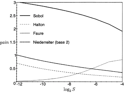
Fig. 6. Gain for the hybrid sequences compared to the pseudo-Monte Carlo sequence.
the mean square error
S=
v u u t
1
|P|
X
xp∈P
˜
U (xp)−U (xp)
2
for the simulated valuesU˜ and record the results of the simulation atN =2i(i=1, . . . ,17)samples. The evolution
of the mean square errorSis shown in Fig. 4. The pseudo-Monte Carlo sequence is included for comparison. We have also considered the inversive congruential generator (Hellekalek, 1995)
xn+1=858 993 221xn−1+1(mod 2 147 483 053)
instead of the Afflerbach sequence. However, the resulting picture does not differ significantly from Fig. 4 where the Afflerbach sequence is used.
To quantify the effect of using a low discrepancy part in the sequence we perform a regression analysis on the sample results by fitting
log2(S)=Fa1,a2,a3(N )=a0+a1log2(N )+a2log2(log2(N ))+ε (32)
to the data of the log–log plot using least square optimization ofε. Note that the Koksma–Hlawka inequality could be interpreted as implyinga2 = sanda1 = −1. However, we do not seta2 = sas the effective dimension of the simulation may be different to the theoretical dimension and we do not seta2 = −1 as we are using a hybrid sequence. The fitted curves are given in Fig. 5.
We measure the efficiency gain by comparing the regression results. For a given error boundS=S∗we compute the minimal sample sizeN =N∗(sequence)such that the regression error estimate Eq. (32) is lower thanS∗. The required sample size using the hybrid sequences is compared to the required sample size using the pseudo-Monte Carlo sequence. The gain in using the hybrid sequence is expressed as a factorgain=N∗(pseudo)/N∗(hybrid)
of reduction of the required sample size for a given error. Therefore, the pseudo-Monte Carlo sequence takesgain
times the number of samples to reach the same error as the given hybrid sequence. Fig. 6 showsgainas a function of the error bound.
7. Conclusion
We have introduced a model for the ruin problem of a company that is faced with risk proportional to the free reserve. The model may be useful in judging and minimizing credit risk and the risk of international insurance.
An analytic solution is given for the special case of exponentially distributed claims. The series type solution converges quickly and it is thus far superior to the simulation methods. However, if simulation becomes necessary for, e.g. more realistic claim size distributions, our results show that even a small part using the Sobol’ sequence can produce a significant improvement (in our case a factor of 2–3) in the performance of a Monte Carlo simulation. Furthermore, the use of quasi-Monte Carlo alone is no guarantee for good performance if a poor low discrepancy sequence is used.
Acknowledgements
We would like to thank the referee for his valuable comments. The authors were supported by the Austrian Science Foundation (FWF) project 12005.
References
Afflerbach, L., 1990. Die Gütebewertung von Pseudo-Zufallszahlen-Generatoren aufgrund theoretischer Analysen und algorithmischer Berechnungen. Grazer Mathematische Berichte 309.
Beck, J., Chen, W., 1987. Irregularities of Distribution, vol. 89, Cambridge Tracts in Mathematics. Cambridge University Press, Cambridge, New York.
Caflisch, R.E., 1998. Monte Carlo and quasi-Monte Carlo methods. Acta Numerica, 1–49.
Dickson, D.C.M., 1991. The probability of ultimate ruin with a variable premium loading — a special case. Scandinavian Actuarial Journal, 75–86.
Dickson, D.C.M., Gray, J.R., 1984. Exact solutions for ruin probability in the presence of an absorbing upper barrier. Scandinavian Actuarial Journal, 174–186.
Drmota, M., Tichy, R.F., 1997. Sequences, Discrepancies and Applications, vol. 1651, Lecture Notes in Mathematics. Springer, New York. El’sgol’ts, L.E., Norkin, S.B., 1973. Introduction to the Theory and Application of Differential Equations with Deviating Argument, vol. 105,
Mathematics in Science and Engineering. Academic Press, New York.
Faure, H., 1981. Discrépance de suites associées à un système de numération (en dimension un). Bull. Soc. Math. France 109, 143–182. Faure, H., 1982. Discrépance de suites associées à un système de numération (en dimensions). Acta Arithmetica 41, 337–351.
Fishman, G.S., 1990. Multiplicative congruential random number generators with modulus 2β: An exhaustive analysis forβ=32 and a partial analysis forβ=48. Math. Comp. 54, 331–344.
Gerber, H.U., 1981. On the probability of ruin in the presence of a linear dividend barrier. Scandinavian Actuarial Journal, 105–115. Halton, J.H., 1960. On the efficiency of certain quasi-random sequences of points in evaluating multidimensional integrals. Numer. Math. 2,
84–90.
Hellekalek, P., 1995. Inversive pseudo-random number generators: concepts, results and links. In: Alexopolous, C., Kang, K., Lilegdon, W.R., Goldsman, D. (Eds.), Proceedings of the 1995 Winter Simulation Conference, pp. 255–262.
Joy, C., Boyle, P., Tan, K.S., 1996. Quasi-Monte Carlo methods in numerical finance. Management Science 42 (6), 926–938. Kalos, M.H., Whitlock, P.A., 1986. Monte Carlo Methods, vol. I, Wiley, New York.
Morokoff, W.J., Caflisch, E., 1994. Quasi-random sequences and their discrepancies. SIAM Journal of Scientific Computing 15 (6), 1251–1279. Niederreiter, H., 1987. Point sets and sequences with small discrepancy. Monatsh. Math. 104, 273–337.
Niederreiter, H., 1992. Random Number Generation and Quasi-Monte Carlo Methods. SIAM, Philadelphia, PA. Papageorgiou, A., Traub, J., 1996. Beating Monte Carlo. Risk 9, 6.
Paskov, S.H., 1994. Computing high dimensional integrals with applications to finance. Technical Report CUCS-023-94, Columbia Univerisity, New York.
Paskov, S.H., Traub, J., 1995. Faster valuation of financial derivatives. Journal of Portfolio Management, 113–120.
Siegl, T., Tichy, R.F., 1996. Lösungsmethoden eines Risikomodells bei exponentiell fallender Schadensverteilung. Mitteilungen der schweizer Vereinigung der Versicherungsmathematiker, 85–118.
Sobol’, I.M., 1967. On the distribution of points in a cube and the approximate evaluation of integrals. USSR Comput. Math. Math. Phys. 7, 86–112.