Full Terms & Conditions of access and use can be found at
http://www.tandfonline.com/action/journalInformation?journalCode=ubes20
Download by: [Universitas Maritim Raja Ali Haji] Date: 12 January 2016, At: 22:59
Journal of Business & Economic Statistics
ISSN: 0735-0015 (Print) 1537-2707 (Online) Journal homepage: http://www.tandfonline.com/loi/ubes20
A More Timely and Useful Index of Leading
Indicators
Robert H McGuckin, Ataman Ozyildirim & Victor Zarnowitz
To cite this article: Robert H McGuckin, Ataman Ozyildirim & Victor Zarnowitz (2007) A More Timely and Useful Index of Leading Indicators, Journal of Business & Economic Statistics, 25:1, 110-120, DOI: 10.1198/073500106000000279
To link to this article: http://dx.doi.org/10.1198/073500106000000279
Published online: 01 Jan 2012.
Submit your article to this journal
Article views: 91
A More Timely and Useful Index of
Leading Indicators
Robert H. M
CG
UCKIN, Ataman O
ZYILDIRIM, and Victor Z
ARNOWITZThe Conference Board Economics Program, New York, NY 10022 (a.ozyildirim@conference-board.org)
Effectively predicting cyclical movements in the economy is a major challenge. The U.S. leading in-dex (LI) has long been used to analyze and predict economic fluctuations. We describe and test a new procedure for making the LI more timely. The new LI significantly outperforms its older counterpart. It offers substantial gains in real-time, out-of-sample forecasts of changes in aggregate economic activity (real GDP, the index of coincident indicators, and industrial production) and provides timely and accurate ex ante information for predicting not only business cycle turning points, but also monthly changes in the economy.
KEY WORDS: Business cycle; Forecasting; Indicators; Leading index; Times series.
1. INTRODUCTION
Most of the macroeconomic data for the United States re-quire considerable time to collect, process, and release. Lags of 1 month are common for principal monthly indicators. For the quarterly data, the lags are longer. Moreover, many of these indicators are subject to sizeable and time-consuming revisions that presumably reduce measurement errors but add to uncer-tainty and forecasting errors.
The actual recognition lags are considerably longer than these publication lags, because it is difficult to recognize sig-nals in noisy data. As a result, private and public decision and policy makers are faced with long delays and much uncertainty about the current (let alone the future) conditions of the econ-omy. Although government is the main source of macroeco-nomic statistics, its access to the data is not much more timely than that of the public.
At the same time, the publication lags and revision sched-ules vary greatly, and some indicators are available promptly. The U.S. leading index (LI) includes stock prices and inter-est rate spreads that have no significant data lags and relatively few, if any, revisions. The financial market indicators convey a great deal of information with predictive value, yet until re-cently, these indicators were represented in the LI, not by their most recent monthly values, but by their values in the preceding month for which data for other indicators were also available.
This article evaluates a new procedure for calculating the U.S. LI that combines its seven current financial and nonfi-nancial components with simple forecasts of the three remain-ing components that are available only with publication lags. Real-time, out-of-sample tests demonstrate that the new, much timelier LI is superior to the old LI with the same components. Moreover, in contrast to some recent studies, here we show that the LI provides significant ex ante information for predicting changes in total output and other measures of economic activ-ity. Some nonparametric rules and probability model applica-tions of the composite LI performed well in forecasting recent cyclical movements even using real-time data, as reported by Filardo (2004). Other studies question the value of the LI and emphasize selected financial indicators as better predictors of business cycle turning points (Diebold and Rudebusch 1991; Estrella and Mishkin 1998).
Section 2 describes the traditional method of constructing an LI, sets out its rationale, and critiques it. It then discusses the
availability and currency of the components of the old index and provides an outline of the procedures for making the new more timely and useful LI.
Section 3 analyzes the structure of the underlying data and the role of data revisions. It compares the historical LI calcu-lated with the latest available data with successive vintages of the old and new LIs. Using real-time data for each of their com-ponents and holding their composition constant, we make the new and old LIs consistent and comparable, so that their rel-ative predictive capabilities can be strictly assessed. However, the new LI typically involves only 1-month ahead estimates that closely approximate the missing data, which the old LI included in the next month; hence the main difference between the old and the new LIs is the better timeliness of the latter.
Section 4 introduces the current conditions index (CCI), which the LI is designed to predict. It asks how well the LI pre-dicts the historical and the real time estimates for CCI and real gross domestic product (RGDP). The former are values taken after all revisions of the data, whereas the latter are the pub-lished values on the date to which the original forecast applied. To establish benchmarks for evaluating the value of the time-lier LI, we specify a broad class of linear models to test the LI’s performance in forecasts of growth rates of CCI and RGDP. Using growth rates of the CCI and RGDP is in the spirit of the indicator approach and, as a practical matter, is essential be-cause there is very little difference in the ability of the new and old LIs to distinguish turning points. We find that both the old LI and the new LI provide improved real-time, out-of-sample forecasts compared with an autoregressive benchmark model. After evaluating the predictive accuracy of the old and new LIs, we modify the model to assess the gains from the more timely LI. Concentrating on the issue of timeliness, we find significant gains to the new procedure.
We conclude in Section 5 by drawing together our findings and placing them in the context of some other related findings in the literature. Because of the large scope of our empirical work and the need to economize on journal space, most of the details of the analysis and measurement is relegated to an appendix, available on The Conference Board website ( www.conference-board.org/economics/workingpapers.cfm).
© 2007 American Statistical Association Journal of Business & Economic Statistics January 2007, Vol. 25, No. 1 DOI 10.1198/073500106000000279 110
2. CONSTRUCTION OF THE COMPOSITE LEADING INDEX
2.1 Logic and Consequences of the Traditional Method
The indicators used to construct the LI tend to move ahead of the business cycle as represented by the monthly coincident indicators and the quarterly RGDP; for example, businesses adjust hours before changing employment by hiring or firing, and new orders for machinery and equipment are placed before completing investment plans. Thus, by design, the composite index of leading indicators should help predict changes in real economic activity.
Business cycles vary in duration, magnitude, and conse-quences largely because their specific sources differ over time. The multicausal, multifactor nature of the economic move-ments helps explain why the LI works better over time than does any of its individual components: the average workweek, initial claims for unemployment insurance, new investment commitments (orders, contracts, housing permits), real money supply, yield spread, stock prices, and consumer expectations. The leading series themselves vary in terms of timing, smooth-ness, currency, and other features. The index gains from this di-versification. However, many technical problems arise from this diversity, perhaps none more vexing than those stemming from the fact that some indicators are available promptly, whereas others are available only with substantial lags.
The indicator approach, one of several techniques of busi-ness cycle analysis, has been a major component of the Na-tional Bureau of Economic Research (NBER) program since the work of Burns and Mitchell (1946). The NBER, the Bureau of Economic Analysis (BEA) of the U.S. Department of Com-merce, and, until recently, The Conference Board successively used the traditional method. It incorporated two rules. First, all components of the LI refer to the same month. Second, only actual data—no forecasts—are used. This long-followed pro-cedure had its logic. The dataset used was time-consistent, be-cause it covered the same period, as is usual in LI construction. In addition, because it consisted of actual data, the LI avoided errors inevitably associated with forecasting.
However, this methodology suffered from failing to use the latest available financial and other data with presumably more relevance and more predictive value than the data actually used, which were 1 month older. Although forecasting the missing variables introduces error, it also improves the timeliness of the composite index.
The old procedure had no good way to cope with the serious problem of missing data. The prevailing practice was to cal-culate the LI with a partial set of components, for example, a minimum of 40–60% depending on the country accord-ing to the Organization for Economic Cooperation and De-velopment (OECD) (see Nilsson 1987; also see http://www. oecd.org/std/li1.htm). An equally arbitrary rule of at least 50% of components was used in the United States until recently. Al-though any such rule allowed the LI to be more up to date, all raised serious problems. First, there was a very undesirable trade-off between the coverage and timing of the LI: the more complete the coverage, the less timely the LI. Second, without a full set of components, the volatility adjustment
(standardiza-tion) factors used to calculate the contributions of the compo-nents often changed dramatically depending on which series, and how many of them, were missing.
The only effective way to avoid these problems while adher-ing to the rules of the traditional method was to delay issuadher-ing the LI until preliminary data became available for all of its com-ponents. For the monthly indicators used in the most recent ver-sion of the traditional LI, this meant a production lag of almost 2 months.
2.2 The Gain in Timeliness From the New Method
In the old procedure, the LI released during the current month(t)referred to the month(t−2). In the new procedure, implemented by The Conference Board since January 2001, the LI released in the same month(t)refers to the month(t−1). For example, the old LI would be calculated in the first week of March(t)for January(t−2), the month with a complete set of components, whereas the new LI is calculated in the third week of March for February(t−1), the month for which 70% of the components are available and 30% are forecast. Before the in-troduction of the new method, users of the indicator approach had to wait for 2 more weeks until April for the February LI. This is a major gain in timeliness in a world where business and government analysts revise and update their predictions nearly every week.
LetYbe the vector of indicator series with data lags such that they are not available in the current publication period. Vari-ables in Y are generally data on real macroeconomic activity and price indexes. Specifically, for the present U.S. LI, these in-clude new orders for consumer goods and materials, new orders for nondefense capital goods, and real money supply. (Nominal money supply is available, but the personal consumption expen-diture deflator used to adjust it is not.)
LetX be the vector of the indicator series available for the most recent complete month. These include the promptest fi-nancial indicators such as stock prices, bond prices, interest rates, and yield spreads. They also include many other, less prompt but frequently reported series. Seven of the 10 compo-nents of the U.S. LI fall into this category.
A simple formalization of the old and new indexing proce-dures may be given as represents the value of the LI for the montht−ipublished in the montht, whereidenotes the publication lag. The first sub-script in the LI gives the month of release; the second subsub-script, the month of the target of the forecast or the reference data. The symbol ˆ refers to a magnitude based at least in part on
some kind of forecasting. Herein we take I(·)to be fixed and identical to The Conference Board’s indexing procedure. The Conference Board follows long-standing practice of using stan-dardization factors to equalize the volatility of the LI compo-nents so that relatively more volatile series do not exert undue influence on the LI (for details of indexing, see The Conference Board 2001.)
2.3 The Costs and Benefits of the New Procedure
The old LI performed its forecasting function with errors due largely to missing data and other measurement problems. In the new LI, some of these problems are reduced, but new errors are introduced by the forecasts ofYˆt−1.
UsingXt−1instead ofXt−2results in a substantial advantage
of greater timeliness, because the new LI is available more than half a month earlier than the corresponding old LI. Thus, for the new procedure to be preferred, it is only necessary that the er-rors ofLIˆnewnot be so large as to negate that advantage. In other words,LIˆnewmust do a better job of forecasting the economy thanLIold. Although not assured, this is likely for the following reasons. First, theYˆt−1forecasts are typically short, and hence
they should produce relatively small errors. Second, the individ-ual errors of the components of the vectorYˆt−1may offset one
another when combined to form the composite index. Third, for any forecast horizon, the new LI will be 2 weeks closer to it.
The Yˆt−1 forecasts for the United States are restricted to
1-month-ahead forecasts, but for other countries, multistep forecasts for someY variables are necessary. In most foreign countries there are fewer weekly and monthly and more quar-terly and annual series, and for this and other reasons the lags tend to be longer, up to 3–5 months. Hence, the need for the new procedure is even greater outside the United States than for the United States, although the potential errors from forecasting the
Y variables are greater as well.
Of course, there are numerous ways to forecastYt. However, the advantages of simplicity, stability, and low cost argue for concentrating on easily implemented autoregressive models. Of these, the simple second-order model excelled and was adopted after passing some fairly strict tests. For practical reasons asso-ciated with production of the LIs on a monthly basis, frequent changes in the forecast model are avoided, and The Conference Board uses the same model for fixed periods of at least a year or two, but reestimates it every month (see McGuckin, Ozyildirim, and Zarnowitz 2001).
3. COMPARING THE LEADING INDEXES AND THEIR
PREDICTIVE TARGETS
3.1 Calculating the New and Old Indexes in a Consistent Manner
To compare the new and old LIs on a consistent basis, we calculated the LIs using real-time data for each of the 10 series that compose the current LI published monthly by The Con-ference Board. This puts the new and old LIs on strictly equal footing, eliminating all changes in composition or methodology (e.g., base years, standardization factors) and hence all possible discontinuities or differences due to these factors.
The important issue of the consequences of changes in the composition of the LI has been treated in a separate article. McGuckin and Ozyildirim (2004) found that revisions to the components of the LI are typically undertaken because of data problems (e.g., discontinued series or quality deterioration) and to account for changes in economic structure. These revi-sions generally resolve the problems with the data or structural changes. However, our present task of evaluating the new LI
relative to the old, less timely LI calls for tests of composite in-dexes with identical, constant composition; the past changes in index composition are not material to this task.
The real-time data used in this study were first electronically archived in 1989 by the former Statistical Indicators Division of the U.S. Department of Commerce and, since 1995, by The Conference Board. The data available in January 1989, called the “January 1989 vintage,” consist of a monthly sample cover-ing the period January 1959–November 1988. Each consecutive monthly vintage adds the next month’s observation. The dataset used in this article covers vintages from January 1989 through September 2002. Hence 165 vintages and 165 corresponding sets of data are used to create an equal number of versions of the LI, each starting in January 1959.
3.2 Comparing the Old and New Indexes
Figure 1 plotsLIˆnewfor the period December 1988–August 2002 andLIoldfor November 1988–July 2002. Each point on the graph, for both the new LI and the old LI, represents the end value of one of the 165 vintages of data. In addition, Fig-ure 1(a) shows the “historical LI,” that is, the last vintage that in-corporates all revisions to date. Note that the chart provides the data for the old and new LIs for the same month, even though the new LI would be published somewhat earlier. Section 4.5 amends the analysis to assess the improvement from timeliness. By construction, any difference between the old and new LIs must be due to the effects of data revisions and forecasting the missing data. But at any time, historical postrevision values ac-count for the great bulk of all observations and are generally identical in the different vintages. Forecasts for missing data apply only to the most recent values (end months for each vin-tage) of three of the components of LI. This explains why the differences between the vintages tend to be so limited.
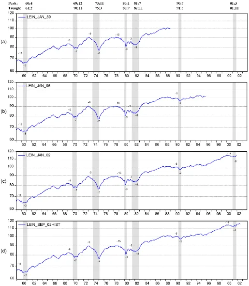
The historical index deviates from both the old LI and the new LI by much more than these LIs deviate from each other, but mainly in the level, not in the pattern of cyclical change, which is shared by all three series. This is well illustrated in Figure 1 for the period since 1989, which covers two recessions and the long expansion between them. But it applies to the en-tire period 1959–2002 with its seven business cycles, as shown in Figure 2. The patterns of cyclical change are virtually iden-tical in the different vintages of the new LI; moreover, even the short irregular fluctuations appear very similar. The successive vintages show an upward tilt. For example, the historical index, which is the last vintage (September 2002), shows the strongest upward trend. Underestimation of growth and inflation appears to be a frequent characteristic of preliminary data in long expan-sions like the 1960s and 1990s (cf. Zarnowitz 1992, chap. 13).
Figure 1(b) shows the percent differences between the two real-time level series plotted in Figure 1(a). It is evi-dent that these differences are very small most of the time;
ˆ
LInewandLIold practically overlap. Further, the time series of the differences is essentially random and has little if any bias; the positive and negative differences balance out each other.
The randomness of the differences between the old LI and the new LI is a welcome feature, because it means that fore-casting the missing components of the index introduces no net systematic error; so is the fact that the discrepancies are gen-erally small (fractions of 1%). This suggests that any errors
(a)
(b)
Figure 1. Old and New Composite LIs, November 1988–August 2002. (a) Index (1987=100) ( , new LI; , old LI; , historical LI). (b) Percent ( , ratio, old to new). Mean, .027244; standard deviation, .227264.
caused by the new procedures are likely to be more than offset by improved timeliness. Nonetheless, the differences in timing between the two indexes occasionally cause them to differ sig-nificantly because of large benchmark revisions in some com-ponents; in a few scattered months,LIˆnewuses prebenchmark data, whereasLIolduses postbenchmark data.
Figure 1 also shows that the old and new real-time leading composites available since 1989 can hardly be distinguished by their cyclical timing. This, too, is good news, because it confirms the robustness and validity of our dating procedure. Because their cyclical timing is essentially identical, the new and old LIs cannot be distinguished by how well they antici-pate the onset of business cycle recessions and recoveries. With the same composition, they face the same data and produce the same leads. But the new procedure reduces the delays involved in publication and results in a timelier index, which should prove helpful in actual recognition of turning points. Because differences in forecasting the turning points are not an issue, all tests are based on how well the new LI versus the old LI does in forecasting times series that represent total economic activ-ity. These tests are both more general and more demanding than turning point comparisons; they use a regression framework and distinguish quantitatively between historical and real-time data.
4. HOW WELL DOES THE LEADING
INDEX PREDICT?
4.1 Data, Testing Standards, and Procedures
The LI is widely used as a tool to forecast changes in the di-rection of aggregate economic activity, particularly the business
cycle turning points, whose dates are determined historically by the NBER. In this task, the NBER relies to a large extent on the monthly coincident indicators, which together constitute the CCI: nonfarm establishment employment, real personal income less transfers, real manufacturing and trade sales, and industrial production. Hence business cycle peaks and troughs are well approximated by the dates of peaks and troughs in the CCI (for details, see Zarnowitz 2001). This is documented in Figure 3, which also shows that the LI leads the CCI at all business cycle peaks and troughs, and that the CCI and RGDP, which is the most comprehensive measure of U.S. output, are very closely associated.
Because our principal purpose is to compare the accuracy of monthly forecasts, a true monthly index such as the CCI is a particularly appropriate target measure of economic activity to be predicted. The LI was developed to predict the CCI, and the relationship between the two composite indexes is of major an-alytical interest. The CCI is composed of several variables (not just output), all of which cover important economic activities. The RGDP is subject to long strings of revisions, which are of-ten large; the CCI is revised less, partly because the revisions of its components frequently offset each other. Researchers often use the LIs to predict changes in industrial production (IP), par-ticularly in Europe. These forecasts perform well. But because IP covers a relatively small and declining part of the economy (manufacturing, mining, and utilities), we report tests based on IP only in an appendix available on The Conference Board’s website.
Although these points argue in favor of using the CCI rather than the RGDP, because of the interest in and importance of
Figure 2. Historical LI (as of September 2002) and Three Selected Vintages of the New LI, January 1959–August 2002.
the RGDP as a comprehensive measure of economic activity, we undertake tests with both variables. Because no reliable monthly RGDP data are available (estimates of monthly RGDP by Macroeconomic Advisers, a private forecasting firm, are limited to the 1990s and are not widely accepted), we work with quarterly LI, even though this transformation causes a
consid-erable loss of information. Alternatively, interpolations of quar-terly to monthly RGDP to take advantage of the fact that the leading indicators are monthly can adversely affect the results. This is because the interpolations arbitrarily smooth RGDP, which is the series used both as the dependent variable and, lagged, as one of the explanatory variables. The results
Figure 3. U.S. Current Conditions Index, U.S. Leading Index and Real GDP January 1959–August 2002. The shaded areas represent U.S. busines cycle recessions as dated by the National Bureau of Economic Research. The latest shading relates to the recession of 2001 and is dated according to the cyclical contraction of the CGI (the U.S. current conditions or coincident index). P denotes the specific-cycle peaks and T the troughs in the Leading and Current Conditions Indexes. The numbers at the P and T markings denote the leads or lags in months at the business cycle peaks and troughs respectively.
lish the usefulness of the LI as a forecasting tool for both the CCI and the RGDP; the LI adds important information to fore-casts of growth in either measure of economic activity. It is par-ticularly important to know that the LI improves forecasts of the CCI, because the procedure for making the LI timelier is best evaluated with high-frequency monthly data.
In determining whether the LI (old or new) adds useful in-formation to forecasts of basic measures of aggregate economy, we use the following standard: LI should improve on simple au-toregressive forecasts for the monthly and quarterly measures of aggregate activity such as IP, CCI, and RGDP. We first con-firm the well-known and much-tested finding that the historical LI improves on the autoregression of the target variable. This has been done in an earlier version of this study (McGuckin et al. 2001, pp. 15–19) and is not restated here. We then compare the old and new leading LIs using out-of-sample, real-time tests that ignore the potential gains from the greater timeliness of the new LI. This provides a good benchmark for isolating the gains to timeliness in Section 4.5.
The regressions have the same structure for each vintage and are used to create a sequence of forecast errors based on dif-ferences between the predicted and the historical values of the corresponding actual growth rates in the target economywide aggregate. The mean squared error (MSE) is our preferred mea-sure of accuracy. The same procedure is applied in a series of exercises that vary the forecast horizons (1, 3, or 6 months ahead), spans over which growth is measured in the estimating equation (1, 3, 6, or 9 months) the number of lags in the depen-dent variables (1, 3, 6, or 9) for CCI forecasts. In RGDP fore-casts, the horizons vary from 1 to 2 and 3 quarters, the growth
rate spans vary from 1 to 2, 3, and 4 quarters, and the number of lagged terms varies from 1 to 2, 3, and 4.
The forecast regression models are specified in changes in natural logarithms for all variables: RGDP, the coincident in-dex, and the LIs. This conforms to the way in which analysts generally use the recent growth rates in the LI to detect signals regarding the direction of economic activity. In addition, it also avoids spuriously high correlations due to common trends that obtain in the levels of the indexes. As noted by Camacho and Perez-Quiros (2002, pp. 62–63), the augmented Dickey–Fuller test cannot reject the null hypothesis of a unit root in the levels of the LI series, but is consistent with stationarity of log differ-ences of LI.
All of our tests use as predictors exclusively real-time data that would have been available to the contemporary forecaster at the time. [Real-time data were obtained from the website of the Federal Reserve Bank of Philadelphia for RGDP (see Croushore and Stark 2001) and for the CCI and LI from The Conference Board.] This has the advantage of reproducing with reasonable fairness the actual forecasting situation.
For both RGDPt andCCIt, two alternative versions of the variable are forecast. One version uses the historical (i.e., re-vised data available at present), and the other uses the real-time data (i.e., the preliminary estimates available soon after the forecast). The latter approach is more realistic and tends to produce smaller errors because it absolves the forecaster from predicting the cumulative effects of future revisions of the data (which may or may not be predictable). However, using the his-torical target data follows a rather common practice of requiring the forecaster to use preliminary estimates to predict data
corporating future revisions in the target variable. Thus the first approach allows a comparison of our results to those from other studies that pursue the same strategy (see in particular Diebold and Rudebusch 1991). The revised data are believed to be closer to the truth. The use of revised data in lagged values of the de-pendent variable gives the autoregressive element an advantage compared with the contribution of the LI term, which is based on preliminary data. Assessments of the forecasts thus mix fore-casting and measurement errors, which makes it more difficult for the LI to improve the forecast (see also Amato and Swan-son 2001; Croushore and Stark 2002; RobertSwan-son and Tallman 1998).
4.2 Testing Models Formalized
To give the models a formal representation, letjxmt (jxqt) denote the growth rate of CCI (RGDP) over the pastjmonths (quarters) ending in month (quarter)t. To provide a standard for evaluating the forecasting power of the LI, a simple autore-gressive equation is used as a benchmark in whichjxmt (jxqt)
Consider, for example, the benchmark equation for the monthly CCI, which takes the form
jCCIt=α1+
There follow tests of whether adding lags of the old or new LI to this equation reduces out-of-sample forecast errors. Equa-tion (4) adds lags of the old LI to the benchmark equaEqua-tion (3),
jCCIt=α2+
Equation (5) adds lags of the new LI instead,
jCCIt=α3+
This gives 16 different combinations of the spans of growth rates (j) and number of lags (k) for each of the foregoing three models. We repeat the same exercise for forecasts 3 and 6 months ahead (p=4 and 7). This provides us with 48
fore-cast exercises classified by three factors: the length of forefore-cast horizon, the number of the lagged explanatory terms, and trans-formation of the data (span of the growth rates). Using analo-gous equations in the quarterly frequency, we undertake also 48 forecast exercises for the RGDP.
No effort was made to optimize the predictive regression specifications (this belongs in another article). Rather, we tried to get a sufficiently comprehensive and diverse picture of what the alternative LIs—historical and real time, old and new—can contribute, even under relatively unfavorable conditions. This approach—looking at a broad and symmetric set of models— was modified in one way; only results for models for which the span of growth in the variables in the model is greater than or equal to the forecast horizon are reported. Longer forecasts are not well served by short growth rates, and using short spans in the longer forecasts provided unreliable results.
4.3 Out-of-Sample Forecasts of Changes in RGDP
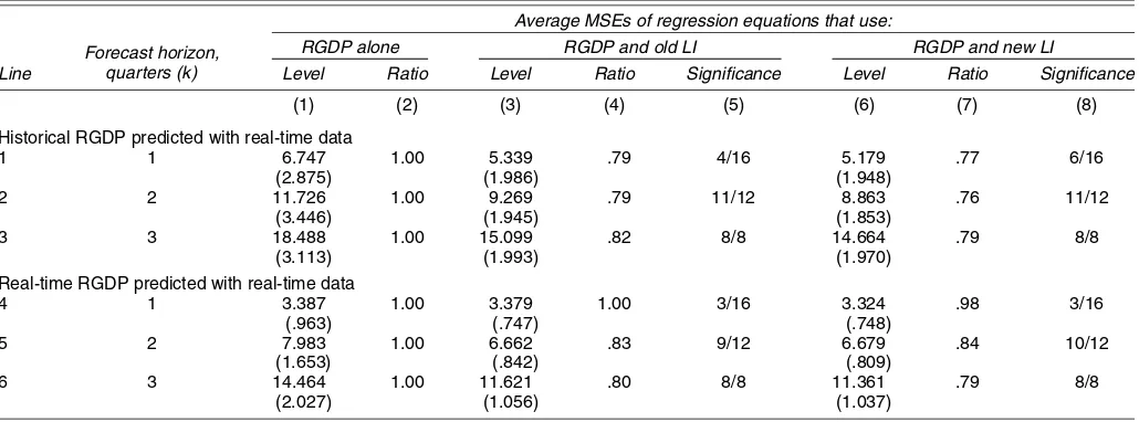
4.3.1 Models With LI versus Autoregressive Models. Ta-ble 1 gives the MSEs averaged across all corresponding equa-tions used to compute the forecasts of the growth rates of RGDP. Columns 1 and 2 refer to the 1-, 2-, and 3-quarter-ahead forecasts of the benchmark autoregressive model. Next, in the same order, are the results for the models that add the old LI (columns 3–5) and the new LI (columns 6–8). Columns 3 and 6 show the average levels of the MSEs across the models in each horizon. Columns 4 and 7 show the ratios of these summary er-ror measures to the corresponding number for the autoregres-sive model, which is set equal to 1 in column 2. Entries in columns 5 and 8 are the number of models in each category in which adding the LI to a forecast equation has significantly reduced the out-of-sample errors at the 5% level.
The main finding of Table 1 is that the autoregressive forecast errors are reduced significantly by the addition of the LI terms in each line (i.e., on the average across all models for each hori-zon), regardless whether the target is the historical or the real-time RGDP growth rate. Using new LI data reduces the errors slightly more than using the old LI in five of the six cases (com-pare columns 4 and 7, remembering that the lower the ratio, the greater the error reduction). The only exception is the 2-quarter-ahead forecast of real time RGDP growth rate (line 5), where the addition of a new LI team produces a minutely smaller im-provement than the addition of an old LI term.
Real-time data predict real-time RGDP growth rates much more accurately than they predict historical RGDP growth rates. The average MSEs in lines 4–6 are 22–50% lower than the corresponding entries in lines 1–3. This is what one would expect, because, as hinted earlier, forecasting the measurement errors to be eliminated by the future RGDP revision is probably a difficult and possibly impossible task. (These errors should be largely random or else they could have been predicted by the compilers of the national income and product accounts them-selves.) The contributions of the LI terms are larger in lines 1 and 2 than in lines 4 and 5, but larger in line 6 than in line 3. The leading indicators are more helpful in the intermediate forecasts than in the shortest forecasts, and the noisy measure-ment errors (as estimated by the data revision) hurt the shortest forecasts the most.
4.3.2 Significance Tests. Our tests involve comparing the predictive accuracy in nested models (i.e., an autoregressive model vs. an alternative obtained by adding the LI). There-fore, a standard test of predictive accuracy, such as the popu-lar Diebold–Mariano (DM) test (Diebold and Mariano 1995),
Table 1. Out-of-Sample Forecasts of Log Changes in U.S. RGDP: Forecast MSEs for Autoregressive Benchmark Models and for Models With the LI, 1989 Q1–2002 Q3
Average MSEs of regression equations that use:
Forecast horizon, quarters (k )
RGDP alone RGDP and old LI RGDP and new LI
Line Level Ratio Level Ratio Significance Level Ratio Significance
(1) (2) (3) (4) (5) (6) (7) (8)
Historical RGDP predicted with real-time data
1 1 6.747 1.00 5.339 .79 4/16 5.179 .77 6/16
(2.875) (1.986) (1.948)
2 2 11.726 1.00 9.269 .79 11/12 8.863 .76 11/12
(3.446) (1.945) (1.853)
3 3 18.488 1.00 15.099 .82 8/8 14.664 .79 8/8
(3.113) (1.993) (1.970)
Real-time RGDP predicted with real-time data
4 1 3.387 1.00 3.379 1.00 3/16 3.324 .98 3/16
NOTE: The entries in columns 1, 3, and 5 are averages of the MSEs in each category (16 fork=1, 12 fork=2, and 8 fork=3, wherekis the forecast horizon in quarters); those in parentheses are the corresponding standard deviations of the MSEs in each category. The entries in columns 2, 4, and 6 are ratios, the average MSE in each class is divided by its counterpart for the autoregressive model. Real-time data on RGDP was obtained from the website of the Federal Reserve Bank of Philadelphia (see Croushore and Stark 2001). Entries in columns 5 and 8 are the number of models in each category where the LI has significant forecast ability at the 5% level. Significance results are based on the Mp test statistic (CCS) developed by Chao et. al. (2001). An alternative test statistic proposed by Clark and McCracken (2001) gave similar results. The detailed results for both test statistics in each forecast model are reported in the appendix on The Conference Board website’s appendix (see endnote 2).
is not appropriate, because under the null of equal predictive ability, the limiting distribution of the DM test is not normal (see McCracken 2000; Clark and McCracken 2001).
Fortunately, there is a growing literature on significance tests for choosing between nested models (see Corradi and Swanson 2003 for a review.) We used the out-of-sample errors from our forecast models to calculate a test statistic, CCS, developed by Chao, Corradi, and Swanson (2001), which is easy to construct and has a chi-squared distribution with degrees of freedom equal to the number of extra explanatory variables, assuming that the parameter estimation error vanishes. (See also Corradi and Swanson 2002 for a more general version of this test.)
An alternative encompassing test statistic proposed by Clark and McCracken (2001), which is also easy to construct but has a nonstandard distribution, gave similar results. In the summary tables, we report results based on the CCS test, because, unlike the Clark and McCracken test, it is applicable to all forecast horizons. Moreover, the CCS test is robust to dynamic mis-specification. The detailed results for both test statistics in each forecast model and horizon combination are reported in the ap-pendix available on The Conference Board website, as men-tioned in Section 1.
For 1-quarter-ahead forecasts, the addition of old LI low-ers the forecast errors significantly at the 5% level for only 4 of the 16 models (see line 1, column 5). The addition of the new LI does only a little better, reducing the errors significantly for 6 of the 16 models (line 1, column 8). This is so when his-torical RGDP is predicted; for real-time RGDP, the results are worse, with 3 of the 16 models gaining from the addition of either the old LI or the new LI terms. However, significant im-provements are obtained for as many as 11 of the 12 models, for the 2-quarter-ahead and for all 8 models for the 3-quarter-ahead forecasts of historical RGDP with both the old and new LIs (see lines 2 and 3, columns 5 and 8). The results for predict-ing real-time RGDP are almost as positive for the 2-quarter-ahead forecasts and equally positive for the 3-quarter-2-quarter-ahead
forecasts (lines 5 and 6). This provides additional evidence that the leading indicators are particularly valuable for predictions over longer horizons.
4.4 Out-of-Sample Forecasts of Changes in the Current Conditions Index
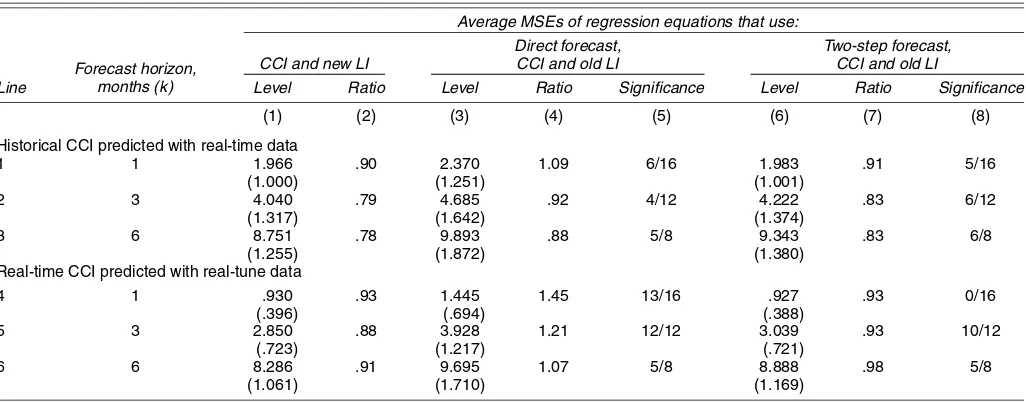
4.4.1 Models With LI versus Autoregressive Models. Ta-ble 2, which has the same format as TaTa-ble 1, demonstrates that the U.S. LI systematically improves on the autoregres-sive benchmark model for the CCI. The overall MSEs (aver-ages for 1-month-ahead, 3-month-ahead, and 6-month-ahead predictions) are substantially lower for the regressions with lagged CCI and LI terms than for the regressions with lagged CCI terms only. This is true not only for the real-time old LI (columns 3 and 4), but also for the new LI, even when the time-liness advantage of the latter is ignored (columns 6 and 7).
Again, in each case the entries in odd columns of part B are lower than the corresponding entries in part A: real-time data predict real-time CCI more accurately than they predict re-vised historical CCI. This parallels our finding for RGDP in Ta-ble 1. Also, adding LI lowers the forecasting errors compared with those of the autoregressive benchmark models more for the comparisons with the historical target series than for the comparisons with the real-time target series (cf. the ratios in columns 4 and 7). Unlike Table 1, Table 2 shows no exceptions from the latter rule. The appendix on The Conference Board website reports all of the underlying details and lists the MSEs for all of the forecast exercises.
4.4.2 Significance Tests. The tests of significance summed in Table 2, columns 5 and 8, also parallel those in Table 1 in terms of format and results. Again, they are the weakest for the shortest forecasts, especially so when real-time CCI growth for the next month is predicted (cf. lines 1 and 4). For 3-month-ahead forecasts, LI decreases the errors from the
Table 2. Out-of-Sample Forecasts of Log Changes in the CCI: Forecast MSE, for Autoregressive Benchmark Models and for Models With the LI, January 1989–October 2002
Average MSEs of regression equations that use:
Forecast horizon, months (k )
CGI alone CCI and old LI CCI and new LI
Line Level Ratio Level Ratio Significance Level Ratio Significance
(1) (2) (3) (4) (5) (6) (7) (8)
Historical CCI predicted with real-time data
1 1 2.182 1.00 1.945 .89 9/16 1.966 .90 8/16
Real-time CCI predicted with real-time data
4 1 .997 1.00 .914 .92 3/16 .930 .93 3/16
NOTE: The entries in columns 1, 3, and 5 are averages of the MSEs in each category (16 fork=1, 12 fork=3, and 8 fork=6, wherekis the forecast horizon in months); those in parentheses are the corresponding standard deviations of the MSEs in each category. The entries in columns 2, 4, and 6 are ratios, the average MSE in each class is divided by its counterpart for autoregressive model. Real-time data on the CCI are obtained from The Conference Board archives. Note that because of methodological changes in 1993 and 1997, we have reconstructed the real-time CCI using real-time data for 1989–1996 vintages but with the current methodology to match the vintages from 1997–2002. (See “Business Cycle Indicators: Upcoming Revision of the Composite Indexes,” Green and Beckman 1993, pp. 44–51, and The Conference Board 2001, p. 57.) Entries in columns 5 and 8 are the number of models in each category where the LI has significant forecast ability at the 5% level. Significance results are based on the test statistic (CCS) developed by Chao et. al. (2001). An alternative test statistic proposed by Clark and McCracken (2001) also gave similar results. The detailed results for both test statistics in each forecast model are reported in the appendix on The Conference Board website’s appendix (see endnote 2).
autoregressive models in all but 1 of the 24 cases; for 6-month-ahead forecasts, LI is successful in all 16 cases.
We conclude that the leading indicators display greater net predictive power over longer horizons. They also improve on the autoregressive benchmark forecasts more when historical targets are used than when real time targets are used. All of this applies to the CCI forecasts, as well as to the RGDP forecasts.
4.5 Improved Timeliness Generates Gains in Forecasting Accuracy
The tests so far have neglected the fact that the target period has a different date for the old LI than for the new LI. For ex-ample, “1-month ahead” means something different for the two indexes; thus to forecast growth in the CCI in March, the old LI requires a 2-month lead (from January), whereas the new LI reaches the same target month in 1 month (from February). The new LI shortens the appropriate forecast horizon, but the shorter the forecast, generally the smaller the forecast errors. We now extend the analysis to evaluate the gains from the earlier release of the LI. To do this, we need to measure explicitly how the two LI forecast the same target period.
As an example, consider a 1-month-ahead forecast for
jCCIt. There are two ways to usejLItold−2to forecastjCCIt. The first is a direct (one-step) prediction in the regression framework:jLIoldt−2andjCCIt−2 are used to jointly predict
jCCIt. The second is a two-step prediction; a second-order autoregressive model is used to estimatejLIoldt−1, and then the
latter value, along withjCCIt−1, is used to predictjCCIt. Table 3 reports the results where the difference in timeliness is accounted for with the old LI and replicates the results for the new LI from Table 2 (columns 6 and 7). The second approach yields somewhat more accurate results, as can be seen in Table 3 (compare columns 3, 4, and 5 with columns 6, 7, and 8).
When the dates of the target months are made identical for the two indexes, the old LI is in effect made to forecast 1 month
further ahead. Therefore, the MSEs of models using the old LI increase substantially (cf. Table 2, column 3 and Table 3, columns 3 and 6). Now the out-of-sample errors of forecasts with the new LI are smaller than the errors of the correspond-ing forecasts with the old LI in 11 of the 12 available compar-isons (cf. Table 3, column 1 with columns 3 and 6; the only exception is in line 4, where the entry in column 6 is slightly less than the entry in column 1). However, the DM tests com-paring the errors of the models using the old LI with the errors of the models using the new LI (columns 5 and 8) indicate that for most of the short forecasts, the differences are not signifi-cant at the 5% level. (Here the alternative models, one with the new LI and the other with the old LI, are nonnested models. The null hypothesis is that the errors from the latter are equal to those from the former. The DM statistic is calculated using the Newey–West heteroscedasticity and autocorrelation consis-tent standard errors with lag truncation equal to 4.) That is, the null hypothesis that the two sets of errors are equal cannot be rejected. Nonetheless, at longer horizons of 3 and 6 months, the performance of the new LI improves, especially when predict-ing real-time CCI; that is, in about two-thirds of the cases, the new LI leads to significantly lower out-of-sample errors. When the difference in timeliness is ignored, both the old and the new LIs lead to similar reductions in mean MSEs (6–10%) com-pared with the benchmark autoregressive model. Based on the DM statistic the null hypothesis that forecast errors are equal cannot be rejected. Compared with the similarity in the forecast accuracy between the old and new LIs when their timeliness is ignored, the results demonstrate that when the same month is targeted by both LIs, the old LI suffers from being less timely than the new LI.
5. CONCLUDING THOUGHTS
The main objective of this article is to evaluate a new proce-dure designed to make more efficient and complete use of the
Table 3. Out-of-Sample Forecasts of Log Changes in the CCI: Forecast MSE, for Autoregressive Benchmark Models and for Models With the LI, January 1989–October 2002
Average MSEs of regression equations that use:
Direct forecast, Two-step forecast, Forecast horizon,
months (k )
CCI and new LI CCI and old LI CCI and old LI
Line Level Ratio Level Ratio Significance Level Ratio Significance
(1) (2) (3) (4) (5) (6) (7) (8)
Historical CCI predicted with real-time data
1 1 1.966 .90 2.370 1.09 6/16 1.983 .91 5/16
Real-time CCI predicted with real-tune data
4 1 .930 .93 1.445 1.45 13/16 .927 .93 0/16
NOTE: See the notes for Table 2. The entries in columns 1, 3, and 5 are averages of the MSEs in each category; those in parentheses are the corresponding standard deviations of the MSEs in each category. The entries in columns 2, 4, and 6 are ratios: the average MSE in each class is divided by its counterpart for the autoregressive model from Table 2, column 1. Entries in columns 5 and 8 are the number of models in each category where the predictive ability of the new LI (column 1) is significantly greater than that of the old LI (columns 3 and 6) at the 5% level. Significance results are based on the DM statistic. The detailed results for the DM statistic for each model in each category are reported in The Conference Board website’s appendix (see endnote 2).
data in the index of leading indicators. A possible reason for the shortcomings of the LI might have been its failure to be as up to date as the financial indicators, which are likely to provide early signals of weakening and downturns in profits and investment and credit commitments. The old procedure had eschewed fore-casting missing data but at the expense of being less complete, less timely, and less accurate.
We specify a workable procedure to temporarily fill the gaps due to data that are missing because of publication lags and show that it provides a better LI. We establish that both the old LI and the new LI provide improved real-time, out-of-sample forecasts compared with autoregressive models that do not use LI information. We then evaluate forecasts for the same calen-dar months using the same procedures. We conclude that the new, timelier LI including the most recent financial data is an improved tool in real-time forecasting environments.
The analysis also suggests that the old, less timely proce-dure offered useful forecasting information. This is an impor-tant step in validating the indicator approach, yet leaves open an important question—what is the best way to incorporate the LI in forecasting equations. Despite the gains to the timelier pro-cedures, the analysis should be extended to nonlinear models. This work should also consider the addition of diffusion indexes and other forms of the leading indicators that are regularly used by practicing forecasters.
ACKNOWLEDGMENTS
The authors thank Phoebus Dhrymes, Jan Jacobs, Chris Sims, Norman Swanson, Peter Zadrozny, The Conference Board Business Cycle Indicators Advisory Panel, seminar participants at the CIRET Conference (2000), the ASA (2002) annual meet-ings, the University of Groningen seminar, Federal Committee on Statistical Methodology Research Conference (2003), and anonymous referees for helpful comments and suggestions. We
would also like to thank Tim Jones for excellent research as-sistance. Any remaining errors are, of course, the authors’. The views expressed in this article are those of the author(s) and do not necessarily represent those of The Conference Board.
[Received January 2001. Revised February 2006.]
REFERENCES
Amato, J. D., and Swanson, N. R. (2001), “The Real Time Predictive Content of Money for Output,”Journal of Monetary Economics, 48, 3–24. Burns, A. F., and Mitchell, W. C. (1946),Measuring Business Cycles, New
York: National Bureau of Economic Research.
Camacho, M., and Perez-Quiros, G. (2002), “This Is What the Leading Indica-tors Lead,”Journal of Applied Econometrics, 17, 61–80.
Chao, J., Corradi, V., and Swanson, N. R. (2001), “An Out-of-Sample Test for Granger Causality,”Macroeconomic Dynamics, 5, 598–620.
Clark, T. E., and McCracken, M. W. (2001), “Tests of Equal Forecast Accu-racy and Encompassing for Nested Models,”Journal of Econometrics, 105, 85–110.
Corradi, V., and Swanson, N. R. (2002), “A Consistent Test for Nonlinear Out-of-Sample Predictive Accuracy,”Journal of Econometrics, 110, 353–381.
(2003), “Some Recent Developments in Predictive Accuracy Testing With Nested Models and (Generic) Nonlinear Alternatives,”International Journal of Forecasting, 20, 185–199.
Croushore, D., and Stark, T. (2001), “A Real-Time Data Set for Macroecono-mists,”Journal of Econometrics, 105, 111–130.
(2002), “Is Macroeconomic Research Robust to Alternative Datasets?” Working Paper 02-3, Federal Reserve Bank of Philadelphia.
Diebold, F. X., and Mariano, R. S. (1995), “Comparing Predictive Accuracy,” Journal of Business & Economic Statistics, 13, 253–263.
Diebold, F. X., and Rudebusch, G. D. (1991), “Forecasting Output With the Composite Leading Index: An ex ante Analysis,”Journal of the American Statistical Association, 86, 603–610.
Estrella, A., and Mishkin, F. S. (1998), “Predicting U.S. Recessions: Financial Variables as Leading Indicators,”The Review of Economics and Statistics, 80, 45–61.
Filardo, A. J. (2004), “The 2001 Recession: What Did Recession Prediction Models Tell Us?” Working Paper 148, Bank of International Settlements. Green, G. R., and Beckman, B. A. (1993), “Business Cycle Indicators:
Upcom-ing Revision of the Composite Indexes,”Survey of Current Business, 73 (10), 44–51.
McCracken, M. W. (2000), “Asymptotics for Out-of-Sample Tests of Causal-ity,” working paper, University of Missouri, Dept. of Economics.
McGuckin, R. H., and Ozyildirim, A. (2004), “Real-Time Tests of the Leading Economic Index: Do Changes in the Index Composition Matter?”Journal of Business Cycle Measurement and Analysis, 1, 171–191.
McGuckin, R. H., Ozyildirim, A., and Zarnowitz, V. (2001), “The Compos-ite Index of Leading Economic Indicators: How to Make It More Timely,” Working Paper 8430, National Bureau of Economic Research.
Nilsson, R. (1987), “OECD Leading Indicators,” Report 9, Organization for Economic Cooperation and Development Economic Studies.
Robertson, J. C. and Tallman, E. (1998), “Data Vintages and Measuring Fore-cast Model Performance,” Economic Review, Fourth Quarter, Federal Re-serve Bank of Atlanta.
The Conference Board (2001),Business Cycle Indicators Handbook, New York: The Conference Board.
Zarnowitz, V. (1992),Business Cycles: Theory, History, Indicators, and Fore-casting, Chicago: The University of Chicago Press, pp. 316–356.
(2001), “Coincident Indicators and the Dating of Business Cycles,” Business Cycle Indicators, 6, 3–4.