A General, Fast, and Robust Implementation of the Time-Optimal Path
Parameterization Algorithm
Quang-Cuong Pham
Abstract—Finding the time-optimal parameterization of a given path subject to kinodynamic constraints is an essential component in many robotic theories and applications. The objective of this paper is to provide a general, fast, and robust implementation of this component. For this, we give a complete solution to the issue of dynamic singularities, which are the main cause of failure in existing implementations. We then present an open-source implementation of the algorithm in C++/Python and demonstrate its robustness and speed in various robotics settings.
Index Terms—Motion planning, optimal control, robot control.
I. INTRODUCTION
Time-optimal motion planning plays a key role in many ar-eas of robotics and automation, from industrial to mobile, to service robotics. While the problem of (optimal)path planning under geometric constraints can be considered as essentially solved in both theory and in practice (see, e.g., [1]), general and efficient solutions to the (optimal)trajectory planning un-der kinodynamic1constraints[2] are still lacking. We argue that time-optimal path parameterization2(TOPP) may constitute an efficient tool to address the latter problem.
There are at least three types of kinodynamic motion planning problems where TOPP is useful or even indispensable. First, some applications such as painting or welding require specifi-cally tracking a predefined path. Second, even when there is no a priorinecessity to track a predefined path, it can be efficient to decouplethe optimal trajectory planning problem into two sim-pler more tractable subproblems: 1) generate a set of paths in the robot configuration space, and 2) optimally time-parameterize these paths and pick the path with the fastest optimal parameter-ization [3], [4]. Third, it was recently suggested that TOPP can also be used to address thefeasibilityproblem [5], i.e., finding onefeasible trajectory in a challenging context, as opposed to
Manuscript received May 21, 2014; accepted August 17, 2014. Date of publi-cation September 11, 2014; date of current version December 3, 2014. This paper was recommended for publication by Associate Editor N. Mansard and Editor A. Kheddar upon evaluation of the reviewers’ comments. This work was sup-ported by “Grants-in-Aid for Scientific Research” for JSPS fellows and by a JSPS postdoctoral fellowship.
The author is with the School of Mechanical and Aerospace En-gineering, Nanyang Technological University, Singapore 639798 (e-mail: [email protected]).
Color versions of one or more of the figures in this paper are available online at http://ieeexplore.ieee.org.
Digital Object Identifier 10.1109/TRO.2014.2351113
1Geometric constraints—such as joints limits or obstacle avoidance—depend
only on the configuration of the robot, while kinodynamic constraints—such as bounds on joint velocity, acceleration, and torque, or dynamic balance—involve also higher order time derivatives of the robot configuration.
2Parameterizinga given geometric path consists in finding a time law to
traverse the path, thereby transforming it into atrajectory.Time-optimal pa-rameterization seeks to minimize the traversal time under given kinodynamic constraints.
selecting an optimal trajectory in a context where it is relatively easy to find many feasible trajectories.
Since the path is constrained, the only “degree of freedom” (DOF) to optimize is the scalar functiont→s(t), which rep-resents the “position” on the path at each time instant. If the system dynamics and constraints are of second order, one can next search for the optimal function in the 2-D space (s,s˙). There are basically three families of methods to do so.
1)Dynamic programming:The first family of methods divide the (s,s˙)plane into a grid and subsequently uses a dynamic programming approach to find the optimal trajectory in the(s,s˙)
plane [6].
2)Convex optimization:The second family of methods dis-cretize only thes-axis (intoNsegments) and subsequently con-vert the original problem into a convex optimization problem in O(N)variables andO(N)equality and inequality constraints [7]–[9]. These methods have the advantage of being versatile (they can, for instance, trade off time duration with other ob-jectives such as energy or torque rate) and can rely on existing efficient convex optimization packages.
3) Numerical integration: The third family of methods are based on the Pontryagin Maximum Principle: The optimal tra-jectory in the(s,s˙)plane is known to be “bang-bang” and can, thus, be found by integrating successively the maximum and minimum accelerations ¨s (see Section II-B for details). This approach is theoretically faster than the previous two, since it exploits the bang-bang structure of the optimization problem (and we shall show that it is indeed faster in practice). However, to our knowledge, there is no available general and efficient im-plementation, perhaps because of the programming difficulties involved by this approach and of the robustness issues asso-ciated with the so-called dynamic singularities[10]–[12]; see details in Section II.
Note that all three families can be applied to a wide variety of robot dynamics and constraints, such as manipulators subject to torque bounds [13], humanoids subject to joint velocity and accelerations bounds [8], [11], mobile robots or humanoids sub-ject to balance and friction constraints [14], [15], nonholonomic robots [16], etc.
The goal of this paper is to provide ageneral,fast, androbust implementation of TOPP. For this, we follow the theoretically faster numerical integration approach. To make it robust, we address the aforementioned critical issue ofdynamic singulari-ties. Such singularities arise in a large proportion of real-world problem instances of TOPP and are one of the main causes of failure of existing implementations of the numerical integration approach. Note that dynamic singularities also cause jitters in the convex optimization approach (see, e.g., [7, Fig. 4]) but are probably not as critical there as in the numerical integration
approach. Yet, in most works devoted to the TOPP algorithm, from original articles [10], [11], [17], [18] to reference textbooks [19], the characterization and treatment of these singularities were not done completely correctly. In Section II, we derive a complete characterization of dynamic singularities and suggest how to appropriately address these singularities. The develop-ment extends our previous contribution in the case of torque bounds (presented at IROS 2013 [12]) to the general case. In Section III, we present an open-source implementation in C++/Python. We show that our implementation is robust and about one order of magnitude faster than existing implemen-tations of the convex optimization approach [7]–[9]. This im-provement is particularly crucial for the global trajectory opti-mization problem or the feasibility problem mentioned earlier, which require calling the TOPP routine tens or hundreds of thou-sands times. Finally, Section IV concludes this paper by briefly discussing the obtained results and future research directions.
II. IMPROVING THEROBUSTNESS OF THENUMERICAL
INTEGRATIONAPPROACH
A. General Formulation of the Time-Optimal Path Parameterization Problem
Let q be ann-dimensional vector representing the config-uration of a robot system. Consider second-order inequality constraints of the form
A(q)¨q+q˙⊤B(q)q˙ +f(q)≤0 (1)
whereA(q),B(q), andf(q)are, respectively, anM ×nmatrix, ann×M ×ntensor, and anM-dimensional vector.
Note that “direct” velocity bounds of the form
˙
q⊤Bv(q) ˙q+fv(q)≤0 (2)
can also be taken into account (see footnote 3 and [20], [21]). Inequality (1) is very general and may represent a large va-riety of second-order systems and constraints. As an example, consider ann-DOF manipulator with dynamics
M(q)q¨+q˙⊤C(q)q˙+g(q) =τ. (3)
Assume that the manipulator is subject to lower and upper bounds on the joint torques, that is, for any jointiand timet,
τim in≤τi(t)≤τim ax.
Clearly, these torque bounds can be put in the form of (1) with
A(q) =
M(q) −M(q)
, B(q) =
C(q) −C(q)
,
f(q) =
g(q)−τm ax
−g(q) +τm in
where τm ax = (τm ax
1 , . . . , τnm ax)⊤, and τm in = (τ1m in, . . . ,
τm in n )⊤.
Consider now a pathP—represented as the underlying path of a trajectoryq(s)s∈[0,se n d]—in the configuration space. As-sume that q(s)s∈[0,se n d] is C
1-and piecewise C2-continuous
(note that how to generate such smooth initial trajectories, espe-cially for closed kinematic chains, is an interesting problem on its own). We are interested in time-parameterizations of
P—or time-reparameterizations of q(s)s∈[0,se n d]—which are increasingscalar functionss: [0, T′]→[0, s
end].
Differentiat-ingq(s(t))with respect totyields
˙
q=qss,˙ q¨=qs¨s+qsss˙2 (4)
where dots denote differentiations with respect to the time pa-rametert, andqs= ddsq andqss= d
2q
ds2. Substituting (4) into (1) then leads to
¨
sA(q)qs+ ˙s2A(q)qss+ ˙s2q⊤sB(q)qs+f(q)≤0
which can be rewritten as
¨
sa(s) + ˙s2b(s) +c(s)≤0 (5)
where
a(s) = A(q(s))qs(s)
b(s) = A(q(s))qss(s) +qs(s)⊤B(q(s))qs(s) (6)
c(s) = f(q(s)).
Equation (5) constitutes another level of abstraction, which is particularly convenient for computer implementation: It suffices indeed to evaluate theM-dimensional vectorsa,b, andcalong the path and feed these vectors as inputs to the optimization al-gorithm. From this formulation, one can also remark that it isnot necessaryto evaluate the full matricesAand tensorsB(which are of sizes M×nandn×M ×n), but only theirproducts (of sizesM) withqsandqss. In the case of torque bounds, the
Recursive Newton–Euler method for inverse dynamics [22] al-lows computing these products without ever evaluating the full
AandB. Finally, this formulation allows very easilycombining different types of constraints: For eachs, it suffices to concate-nate the vectorsa(s)corresponding to the different constraints, and similarly for the vectorsb(s)andc(s).
B. Review of the Numerical Integration Approach
Each rowiof (5) is of the form
ai(s)¨s+bi(s) ˙s2+ci(s)≤0.
There are three cases.
1) Ifai(s)>0, then one hass¨≤ −ci(s)−bi(s) ˙s
2
ai(s) . Define the upper
boundβi= −ci(s)−bi(s) ˙s
2
ai(s) .
2) If ai(s)<0, then one has ¨s≥ −ci(s)−bi(s) ˙s
2
ai(s) . Define thelower
boundαi= −ci(s)−bi(s) ˙s
2
ai(s) .
3) Ifai(s) = 0, thensis a “zero-inertia” point [10], [17].
One then has a certain number of αp and βq. Their total
number is≤M, with equality whensis not a zero-inertia point. One can next define for each(s,s˙)
α(s,s˙) = max
Fig. 1. MVC andα-,β-profiles in the numerical integration approach.
From the above transformations, one can conclude that
q(s(t))t∈[0,T′]satisfies constraints (1) if and only if
∀t∈[0, T′], α(s(t),s˙(t))≤¨s(t)≤β(s(t),s˙(t)). (7)
Note that(s,s˙)→( ˙s, α(s,s˙))and(s,s˙)→( ˙s, β(s,s˙))can be viewed as two vector fields in the (s,s˙) plane. One can integrate velocity profiles following the field( ˙s, α(s,s˙))(from now on, αin short) to obtain minimum acceleration profiles (or α-profiles), or following the field β to obtain maximum accelerationprofiles (orβ-profiles).
Next, observe that ifα(s,s˙)> β(s,s˙), then, from (7), there is no possible value for¨s. Thus, to be valid, every velocity profile must stay below the maximum velocity curve3(MVCin short) defined by
MVC(s)
=
min{s˙≥0 :α(s,s˙)=β(s,s˙)},
ifα(s,0)≤β(s,0)
0, ifα(s,0)> β(s,0).
It was shown (see, e.g., [10]) that the time-minimal velocity profile is obtained by abang-bang-type control, i.e., whereby the optimal profile follows alternatively theβandαfields while always staying below theMVC. More precisely, the algorithm to find the time-optimal parameterization ofPstarting and ending with the desired linear velocitiesvb egandvendis as follows (see
Fig. 1):
1) In the(s,s˙)plane, start from (s= 0,s˙=vb e g/qs(0)) and
inte-grate forward followingβuntil hitting either a) theMVC, in this case go to step 2;
b) the horizontal lines˙= 0, in this case the path is not dynam-ically traversable;
c) the vertical lines=se n d, in this case go to step 3.
2) Search forward along the MVC for the next candidate α→β switch point (cf., Section II-C). From such a switch point:
a) integratebackwardfollowingα, untilintersectinga forward β-profile (from step 1 or recursively from the current step 2). The intersection point constitutes aβ→αswitch point; b) integrateforwardfollowingβ. Then continue as in step 1. The resulting forward profile will be the concatenation of the in-tersected forwardβ-profile, the backwardα-profile obtained in (a), and the forwardβ-profile obtained in (b).
3If “direct” velocity bounds such as in (2) are considered, then they
in-duce another maximum velocity curve, notedMVCd ire c t. In this case, every
velocity profile must stay belowmin(MVC,MVCd ire c t). The treatment of
MVCd ire c twas initiated in [20] and [21] and completed and implemented by
us; see https://github.com/quangounet/TOPP/releases.
3) Start from (s=se n d,s˙=ve n d/qs(se n d)) and integrate back-wardfollowingα, until intersecting a forward profile obtained in steps 1 or 2. The intersection point constitutes aβ→αswitch point. The final profile will be the concatenation of the intersected forward profile and the backwardα-profile just computed.
From the above presentation, it appears that finding theα→
βswitch points is crucial for the numerical integration approach. It was shown in [10], [17], and [18] that a given pointsis an α→βswitch point only in the following three cases:
1) The MVC is discontinuous ats. In this case,s is labeled as a “discontinuous” switch point.
2) The MVC is continuousbutundifferentiableats. In this case,s is labeled as a “singular” switch point or a “dynamic singularity” (previous works labeled such switch points as “zero-inertia points” [18]; however, we shall see below that not all zero-inertia points are singular).
3) The MVC is continuousand differentiableats and the tangent vectorto the MVC at(s,MVC(s))is collinear with the vector
(MVC(s), α(s,MVC(s)))[or, which is the same since we are on the MVC, collinear with the vector(MVC(s), β(s,MVC(s)))]. In this case,sis a labeled as a “tangent” switch point.
Finding discontinuous and tangent switch points does not involve particular difficulties, since it suffices to construct the MVC and examine whether it is discontinuous or whether the tangent to the MVC is collinear withαfor all discretized points salong the path. Regarding the undifferentiable switch points, one approach could consist in checking whether the MVC is continuous but undifferentiable ats. However, this approach is seldom used in practice, since it is comparatively more prone to discretization errors. Instead, it was proposed (cf., [10], [11], and [17]–[19]) to equate undifferentiable points with zero-inertia points, i.e., the points swhere ak(s) = 0for one of the
con-straintsk, and to consequently search for zero-inertia points. This method is, however, not completely correct: We shall see in Section II-C thatnot all zero-inertia points are undiffer-entiable. Thus, only zero-inertia points that are undifferentiable properly constitute singular switch points or dynamic singu-larities. Characterizing and addressing such switch points are of crucial importance since they occur in a large proportion of real-world TOPP instances—they are, in particular, much more frequent than discontinuous and tangent switch points together. Furthermore, sinceαandβfields aredivergentnear these switch points (see Fig. 2), they are the cause of most failures in existing implementations of TOPP.
C. Characterizing Dynamic Singularities
Consider a zero-inertia points∗and assume that it is triggered
by thekth constraint, i.e.,ak(s∗) = 0. Without loss of generality,
we make the assumption thatak(s)<0in a neighborhood to
the left of s∗anda
k(s)>0in a neighborhood to the right of
s∗(the case whena
k switches from positive to negative can be
treated similarly by changing signs at appropriate places). We prove in the Appendix that, if the path is traversable, then ck(s∗)<0. We next distinguish two cases [see Fig. 2(a)].
Case 1: bk(s∗)>0. Defines˙∗=
−ck(s∗)
bk(s∗) . Next, lets˙
† be
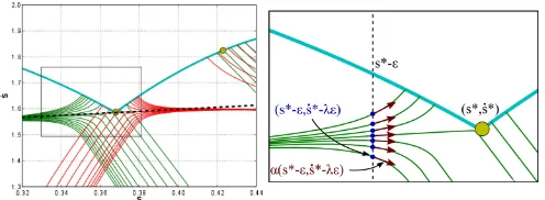
Fig. 2. (a)α- andβ-profiles (in green and red, respectively) near zero-inertia points (yellow points). The left zero-inertia point is a singular switch point, while the right zero-inertia point is not singular. Note that in agreement with the definitions, at any point in the plane, the slope of the red profile is higher than the slope of the green profile, except on the MVC where the two slopes are equal. The dotted line is the line that goes through the switch point and has slopeλcomputed by (10) (cf., Section II-D). (b) Close-up view (zoomed in the black box of (a) centered around the singular switch point.
1) ifs˙†<s˙∗, then constraintkdoesnottrigger a dynamic singularity
ats∗;
2) ifs˙†>s˙∗, then the MVC is indeed undifferentiable ats∗, ands∗
constitutes a dynamic singularity.
Case 2:bk(s∗)<0. We prove that, in this case, constraintk
doesnottrigger a dynamic singularity ats∗.
D. Addressing Dynamic Singularities
1) Previous Treatments: The next difficulty consists in the se-lection of the optimal acceleration to initiate the backward and forward integrations from a dynamic singularitys∗: Indeed the
fieldsαandβare notnaturallydefined at these points because of a division by ak(s∗) = 0. In [17], no indication was given
regarding this matter. In [18], it was stated that “[this] acceler-ation is not uniquely determined” and suggested to chooseany acceleration to initiate the integrations. In [10] (and also in [19] which reproduced the reasoning of [10]), the authors suggested to select the following acceleration to initiate the backward in-tegration (and a similar expression for the forward inin-tegration):
min(α−, α+, αM VC) (8)
where
α−= lim
s↑s∗α(s,MVC(s
∗)), α+ = lim
s↓s∗α(s,MVC(s
∗))
(9)
andαMVC is computed from theslopeof the MVC on the left ofs∗.
However, observing theα-profiles near the dynamic singu-larity of Fig. 2(a), it appears that the definition ofα− in (9) is
arbitrary. Indeed, depending on thedirection from which one moves towards(s∗,MVC(s∗))in the(s,s˙)plane, the limit ofα
is different: for instance, in Fig. 2(a), if one moves from the top left, the limit, if it exists, would be positive, and it would be nega-tive if one moves from the bottom left. In this context, the choice of (9) consisting in moving toward(s∗,MVC(s∗))horizontally
is no more justified than any other choice. More generally, it isimpossibleto extendαby continuity toward(s∗,MVC(s∗))
from the left because theα-profilesdivergewhen approaching
(s∗,MVC(s∗))from the left.
In practice, because of this flow divergence, choosing a slightly incorrect value forαandβ ats∗ may result in strong
oscillations (see Fig. 5), which in turn can make the algorithm incorrectly terminate (because the velocity profile would cross the MVC or the lines˙= 0). In fact, this is probably one of the main reasons of failure in existing implementations.
2) Proposed New Treatment: Fig. 2(b) shows in more detail the α-profiles near a singular switch points∗.
We first show in the Appendix that, if the singularity is trig-gered by constraintk, thenα=αk on the left ofs∗andβ =βk
on the right ofs∗. Consider next the intersections of the vertical
lines=s∗−ǫ, whereǫis an arbitrary small positive number,
with theα-profiles. Anα-profile can reach(s∗,s˙∗)only if its
tangent vectorat the intersectionpoints toward(s∗,s˙∗). This
can be achieved if there exists a real numberλsuch that αk(s∗−ǫ,s˙∗−λǫ)
˙
s∗−λǫ =λ.
Replacingαk by its expression yields the condition
−bk(s∗−ǫ)[ ˙s∗−λǫ]2−ck(s∗−ǫ)
ak(s∗−ǫ)[ ˙s∗−λǫ]
=λ
i.e.,
−bk(s∗−ǫ)[ ˙s∗−λǫ]2−ck(s∗−ǫ) =λak(s∗−ǫ)[ ˙s∗−λǫ].
Computing the Taylor expansion of the above equation at order 1 inǫand recalling that−bk(s∗) ˙s∗2−ck(s∗) = 0andak(s∗) = 0,
one obtains the condition
2λbk(s∗) ˙s∗+b′
k(s∗) ˙s∗2+c′k(s∗) =−λa′k(s∗) ˙s∗.
Solving forλ, one, finally, obtains
λ=− b
′
k(s∗) ˙s∗2+c′k(s∗) [2bk(s∗) +a′k(s∗)] ˙s∗
. (10)
Following the same reasoning on the right ofs∗, one has to
solve
βk(s∗+ǫ,s˙∗+λǫ) ˙
s∗+λǫ =−λ
which leads to the same value as in (10). Thus, the optimal backward and forward acceleration at(s∗,s˙∗)is given by (10).
One can observe in Fig. 2(a) that the black-dotted line, whose slope is given by λ, indeed constitutes the “neutral” line at
(s∗,s˙∗).
Based on the previous development, we propose the follow-ing algorithm when encounterfollow-ing a zero-inertia points∗, with
ak(s∗)<0on the left ofs∗andak(s∗)>0on the right ofs∗. 1) Ifbk(s∗)<0, then constraintkdoes not trigger a singularity.
2) Ifbk(s∗)>0, then computes˙∗ by (11) ands˙†by removing
con-straintkand evaluating again the MVC ats∗.
a) Ifs˙∗>s˙†, then constraintkdoes not trigger a singularity.
b) Ifs˙∗<s˙†, thens∗is a dynamic singularity. Next, computeλ
by (10) and
i) integrate the constant field( ˙s∗,λs˙∗) backwardfor a
small number of time steps. Then, continue by follow-ingα, as in the original algorithm;
ii) integrate the constant field ( ˙s∗,λs˙∗) forward for a
TABLE I
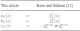
PARAMETERSCORRESPONDENCES This article Kunz and Stilman [11]
ak(s) ↔ fk′(s) bk(s) ↔ fk′′(s) ck(s) ↔ −¨qkm a xorq¨m a xk
Note that after moving a small number of steps away froms∗,
the fieldsαandβbecome smooth so that there is no problem in the integration.
3) About Kunz and Stilman’s Conjecture: Kunz and Stilman [11] were first to remark—in the particular case of TOPP with veloc-ity and acceleration bounds and paths made of straight segments and circular arcs—that the algorithm proposed in [10] could not satisfactorily address dynamic singularities. They conjectured instead that the correct acceleration at the singularity is 0.
From [11, eq. (14)], the correspondences between the pa-rameters of [11] and those of the present article are given in Table I.
Remark that the zero-inertia points in [11] are all located in the circular portions. In such portions, the coefficientsak and
bk have the following form (using our notations):
ak(s) = −
C1
r sin
s
r
+C2
r cos
s
r
bk(s) =
C1
r2 cos
s
r
−C2
r2 sin
s
r
wherer,C1, andC2 are three constants independent ofsin a
neighborhood arounds∗. Differentiatingb
k next yields
b′
k(s) =−
C1
r3 sin
s
r
+C2
r3 cos
s
r
= 1
r2ak(s).
One, thus, hasb′
k(s∗) = 1/r2ak(s∗) = 0at a zero-inertia point.
If this zero-inertia point is actually a dynamic singularity, then, from (10), one obtains thatλ= 0, which proves Kunz and Stil-man’s conjecture.
III. IMPLEMENTATION ANDEVALUATION
A. Open-Source Implementation
We provide an implementation of TOPP in C++ that inte-grates the developments of Section II. We also provide an in-terface in Python for an easy and interactive use. Currently, our implementation supports pure velocity and acceleration bounds, torque bounds, ZMP constraints, multicontact friction constraints, and any combination thereof. The dynamics compu-tations are handled by OpenRAVE [23]. Thanks to the general formulation of Section II-A, new system dynamics and con-straints can be easily added. The implementation and test cases are open-source and available at https://github.com/quangounet/ TOPP/releases.
Fig. 3 illustrates the utilization of TOPP in a multicontact task where a humanoid robot (HRP2, 36 DOFs including the six coordinates of the free-flyer) steps down from a 30-cm-high podium. Velocity and torque bounds were considered for each
Fig. 3. TOPP with velocity, torque, and friction constraints in a multicontact task with the HRP2 robot.(Top) Snapshots of the time-parameterized trajectory taken at equal time intervals. The pink lines represent the contact forces. (Left) (s,s˙)space. Same legends as in Fig. 2. The solid and dotted bold cyan lines are velocity limits that are imposed, respectively, by the torque and friction con-straints [the MVC computed from (1)] and by the “direct” velocity concon-straints [computed from (2)]. The superimposed dotted blue line represents the final (s,s˙)profile, which for some parts followed theα- andβ-profiles and for some other parts “slid” along the “direct” velocity limit. (Right) Normal components of the reaction forces at the front left corner of the left foot (red) and the front left corner of the right hand (green). The normal components were constrained to be≥1N. Note how this constraint was saturated at the foot and hand contact points at different moments in time.
joint, as well as friction cone constraints on the left foot and the right hand (131 inequality constraints in total). The original tra-jectory had a duration of 1 s, and the grid size wasN =100. The time parameterization part (excluding the dynamics computa-tions and the constraints projection step [15]) took 0.005 s on our computer (Intel Core i5 3.2 GHz, 3.8 GB memory, GNU/Linux).
B. Comparison With Previous Treatments of Dynamic Singularities
For this, we tested the algorithm on a model of the 7-DOF Barrett WAM. The velocity and torque bounds are those given by the constructor. Fig. 4 shows a smooth behavior around the dynamic singularity, for both the (s,s˙)profile and the torque profiles.
Next, to demonstrate more clearly the improvements permit-ted by our algorithm, we compared the results given by our algo-rithm and that given by the algoalgo-rithm of [10], which incorrectly proposes to “slide” along the MVC near dynamic singularities. Fig. 5 shows that using the correct acceleration values signifi-cantly decreases the jitters around the dynamic singularity, even at a coarse discretization time step.
Fig. 4. TOPP with velocity and torque constraints for the 7-DOF Barrett WAM. (Top) Snapshots of the time-parameterized trajectory taken at equal time intervals. (Left)(s,s˙)space. Same legends as in Fig. 3. (Right) Torque profiles for shoulder roll (solid red), wrist yaw (solid green), and wrist roll (solid blue). The dotted lines represent the torque bounds in corresponding colors.
Fig. 5. Closeup views of the(s,s˙)profiles and the torque profiles near a dynamic singularity. The computations were done at a time step of 0.01 s. (Left) (s,s˙)profiles. Dotted lines: Profile computed using the method of [10]. Solid lines: Profile computed using our proposed new method. (Right, top) Torque profiles corresponding to the method of [10]. (Right, bottom) Torque profiles corresponding to our method. Note that our method allows suppressing the jitters even at a coarse time step.
TABLE II
TESTING THEIMPLEMENTATION ON1000 TRAJECTORIES System ♯failures ♯singularities WAM torque constraints 0 307 Kinematic constraints 1 539
profiles do not cover the whole segment[0, send][11]—as well
as the number of dynamic singularities encountered in the 1000 instances.
C. Comparison With the Convex Optimization Approach
We first conducted an “informal” comparison of our imple-mentation with the MATLAB-based impleimple-mentations of Ver-scheureet al.[7] and of Debrouwereet al.[9] on the problem of torque bounds. Note that, for the convex optimization part itself, these implementations used a library, YALMIP, which in turn calls an external solver (SeDuMi in [7]), written in C, C++, or
TABLE III
INFORMALCOMPARISON, TORQUECONSTRAINTS
Source Lang. DOF N Exec.
Verscheureet al.2009 [7] MEX 3 299 0.74 s Verscheureet al.2009 [7] MEX 3 1999 2.87 s Debrouwereet al.2013 [9] MEX 7 100 1.5 s
This article C++ 3 300 0.017 s
This article C++ 3 2000 0.10 s This article C++ 7 100 0.0058 s
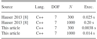
TABLE IV
FORMALCOMPARISON, KINEMATICCONSTRAINTS
Source Lang. DOF N Exec.
Hauser 2013 [8] C++ 7 300 0.025 s Hauser 2013 [8] C++ 7 1000 0.20 s This article C++ 7 300 0.0038 s This article C++ 7 1000 0.014 s
Fortran and precompiled as binary MEX files. Thus, the com-parison with our library written in C++, although “informal,” is not completely unfounded.
Table III gives the convex optimization solver times (which thus do not include the robot dynamics computation times) re-ported in [7] and [9] as well as the running times of our im-plementation after subtracting the robot dynamics computation times. Different grid sizes (N) and number of DOFs to optimize were reported or tested.
Next, in order to make a “formal” comparison on the same computer and using the same programming language, we con-sidered MINTOS (http://www.iu.edu/motion/mintos/, last
ac-cessed December 2013), Hauser’s recent C++ implementation of the convex optimization approach [8], which is, to our knowl-edge, the fastest implementation currently available. To exclude the robot dynamics computations, which are independent of the TOPP problem and whose execution times depend largely on the robot simulation software used, we considered “pure” velocity and acceleration bounds. However, note that, from the general formulation of SectionII-A, these pure kinematic constraints in-volve exactly the same difficulties as any other type of dynamic constraints.
We compiled and ran both implementations on our computer. We considered 1000 random trajectories of dimension 7 and velocity and acceleration bounds as in Section III-B. Table IV reports the average total execution times of the two implemen-tations. It appears from this controlled comparison that our im-plementation is between 7 and 15 times faster than MINTOS.4
IV. CONCLUSION
We have established a rigorous characterization and treatment of dynamic singularities that arise in the numerical integration
4Note that MINTOS includes an innovative “constraints pruning” step that
approach to the TOPP problem. This fully completes the cele-brated line of research on TOPP, which started in the 1980s with the seminal papers of Bobrowet al.[13] and Shin and McKay [6] and which has since then received contributions from many prominent research groups (e.g. [10], [11], [17], [18], just to cite a few).
Based on that contribution and on a general formulation of the TOPP problem, we provided an open-source implementation of TOPP. We showed that this implementation is robust and fast: On typical test cases, it is about one order of magnitude faster than the fastest currently available implementation of the convex optimization approach. As our implementation is open-source and has been designed so as to facilitate the integration of new systems dynamics and constraints, we hope that it will be useful to robotics researchers interested in kinodynamic motion planning.
Our next immediate goal is to attack thefeasibilityproblem (i.e., finding a collision-free dynamically balanced trajectory in a challenging context, in particular, where quasi-static tra-jectories are impossible) for humanoid robots using admissible velocity propagation (AVP) [5], which itself is based on TOPP. We believe that the power of AVP combined with the speed of the present TOPP implementation can make possible the plan-ning of unprecedentedly dynamic motions for humanoid robots in challenging environments.
Finally, from a theoretical perspective, we are investigating how higher order constraints, such as jerk [24], [25] or other types of optimization objectives [7], [9], can be integrated in our TOPP framework.
APPENDIX
CHARACTERIZINGDYNAMICSINGULARITIES
In line with Section C, consider a zero-inertia points∗and assume
thatak(s∗) = 0and thatak(s)<0in a neighborhood to the left of
Note also thatα˜andβ˜are continuous and differentiable in a neighbor-hood arounds∗.
turn, implies that the path is not traversable).
Proof:Suppose that ck(s∗) =η >0. By continuity ofck, there
upper-bounded, in a neighborhood to the left ofs∗. Thus, there exists
a neighborhood to the left ofs∗in whichα(s,0)> β(s,0), which in
turn implies thatMVC(s) = 0in that neighborhood In light of Proposition 2, we assume from now on thatck(s∗)<0.
radical sign is indeed positive. Next, lets˙†be the smallest velocitys˙
that satisfiesα˜(s∗,s˙) = ˜β(s∗,s˙)(s˙†= +∞if no suchs˙exists).
We now distinguish two subcases.
1) Subcases˙†<s˙∗: Lets˙‡= ( ˙s†+ ˙s∗)/2. By the definition of
˙
s∗and the assumption thatb
k(s∗)>0, there existsη >0such that, in
a neighborhood to the left ofs∗
∀s˙≤s˙‡,−b
constraintkdoesnotcontribute toαin a neighborhood to the left ofs∗
and fors˙≤s˙‡. Thus, one hasα= ˜αin a neighborhood to the left of
s∗and fors˙≤s˙‡.
By the same argument, one can show thatβ= ˜βin a neighborhood to the right of s∗ and fors˙≤s˙‡. Combined with Proposition 1, one
has thus obtained thatα= ˜αandβ= ˜β in a neighborhoodaround s∗and fors˙≤s˙‡. This shows that MVC(s∗) = ˙s†, and that the MVC
is entirely determined by α˜ and β˜ around (s∗,s˙†). One can, thus,
conclude that the MVC is continuous and differentiable ats∗, which in
turn implies that constraintkdoesnottrigger a singularity ats∗.
2) Subcase s˙†>s˙∗: Remark first that, excepting degenerate
cases, one can find a neighborhood]s∗−ǫ, s∗+ǫ[×] ˙s∗−η,s˙∗+η[,
in whichα˜is given by a uniqueαqandβ˜is given by a uniqueβp. Note
that, by definition ofα˜andβ, one has˜ p=kandq=k. In the neighborhood just defined, let
u(s) =−ak(s)cq(s) +aq(s)ck(s) One can show similarly that there exists a neighborhood to the right ofs∗in whichMVC(s) = v(s). Combining the results concerning
the left and the right ofs∗, one obtains that theMVCiscontinuousat
s∗, since
However, the MVC isundifferentiableats∗since, in general,
Thus, in this subcase,s∗is indeed a dynamic singularity.
Case bk(s∗)<0: From the assumptions that ck(s∗)<0 and
bk(s∗)<0, one has that−bk(s∗) ˙s2−ck(s∗)>0for alls. Thus, by˙
the same argument as in subcase s˙†<s˙∗, there exists a
neighbor-hood]s∗−ǫ, s∗[whereα= ˜αand a neighborhood]s∗, s∗+ǫ′[where
β= ˜β. One can, thus, conclude that constraint kdoesnottrigger a singularity ats∗.
ACKNOWLEDGMENT
The author would like to thank S. Caron, Z. Shiller and Y. Naka-mura for stimulating discussions regarding TOPP. He is also grateful to S. Caron and R. Diankov for their helps with the implementation.
REFERENCES
[1] S. LaValle,Planning Algorithms. Cambridge, U.K.: Cambridge Univ. Press, 2006.
[2] B. Donald, P. Xavier, J. Canny, and J. Reif, “Kinodynamic motion plan-ning,”J. ACM, vol. 40, no. 5, pp. 1048–1066, 1993.
[3] J. Bobrow, “Optimal robot plant planning using the minimum-time crite-rion,”IEEE J. Robot. Autom., vol. 4, no. 4, pp. 443–450, Aug. 1988. [4] Z. Shiller and S. Dubowsky, “On computing the global time-optimal
motions of robotic manipulators in the presence of obstacles,”IEEE Trans. Robot. Autom., vol. 7, no. 6, pp. 785–797, Dec. 1991.
[5] Q.-C. Pham, S. Caron, and Y. Nakamura, “Kinodynamic planning in the configuration space via velocity interval propagation,” inProc. Robot.: Sci. Syst. Conf., 2013.
[6] K. Shin and N. McKay, “Selection of near-minimum time geometric paths for robotic manipulators,”IEEE Trans. Autom. Control, vol. AC-31, no. 6, pp. 501–511, Jun. 1986.
[7] D. Verscheure, B. Demeulenaere, J. Swevers, J. De Schutter, and M. Diehl, “Time-optimal path tracking for robots: A convex optimization approach,” IEEE Trans. Autom. Control, vol. 54, no. 10, pp. 2318–2327, Oct. 2009. [8] K. Hauser, “Fast interpolation and time-optimization on implicit contact
submanifolds,” inProc. Robot.: Sci. Syst. Conf., 2013.
[9] F. Debrouwere, W. Van Loock, G. Pipeleers, Q. Tran Dinh, M. Diehl, J. De Schutter, and J. Swevers, “Time-optimal path following for robots with convex-concave constraints using sequential convex programming,”IEEE Trans. Robot., vol. 29, no. 6, pp. 1485–1495, Dec. 2013.
[10] Z. Shiller and H. Lu, “Computation of path constrained time optimal motions with dynamic singularities,”J. Dyn. Syst., Meas. Control, vol. 114, pp. 34–40, 1992.
[11] T. Kunz and M. Stilman, “Time-optimal trajectory generation for path following with bounded acceleration and velocity,” inProc. Robot.: Sci. Syst. Conf., 2012, vol. 8, pp. 09–13.
[12] Q.-C. Pham, “Characterizing and addressing dynamic singularities in the time-optimal path parameterization algorithm,” inProc. IEEE/RSJ Int. Conf. Intell. Robots Syst., 2013, pp. 2357–2363.
[13] J. Bobrow, S. Dubowsky, and J. Gibson, “Time-optimal control of robotic manipulators along specified paths,”Int. J. Robot. Res., vol. 4, no. 3, pp. 3–17, 1985.
[14] Q.-C. Pham and Y. Nakamura, “Time-optimal path parameterization for critically dynamic motions of humanoid robots,” inProc. IEEE-RAS Int. Conf. Humanoid Robots, 2012, pp. 165–170.
[15] K. Hauser, “Fast dynamic optimization of robot paths under actuator limits and frictional contact,” inProc. IEEE Int. Conf. Robot. Autom., 2014. [16] F. Bullo and K. M. Lynch, “Kinematic controllability for decoupled
trajec-tory planning in underactuated mechanical systems,”IEEE Trans. Robot. Autom., vol. 17, no. 4, pp. 402–412, Aug. 2001.
[17] F. Pfeiffer and R. Johanni, “A concept for manipulator trajectory planning,” IEEE J. Robot. Autom., vol. RA-3, no. 2, pp. 115–123, Apr. 1987. [18] J. Slotine and H. Yang, “Improving the efficiency of time-optimal
path-following algorithms,”IEEE Trans. Robot. Autom., vol. 5, no. 1, pp. 118– 124, Feb. 1989.
[19] H. Choset, K. M. Lynch, S. Hutchinson, G. Kantor, W. Burgard, L. E. Kavraki, and S. Thrun,Principles of Robot Motion: Theory, Algorithms, and Implementations. Cambridge, MA: MIT Press, 2005.
[20] L. Zlajpah, “On time optimal path control of manipulators with bounded joint velocities and torques,” inProc. IEEE Int. Conf. Robot. Autom., 1996, vol. 2, pp. 1572–1577.
[21] F. Lamiraux and J.-P. Laumond, “From paths to trajectories for multi-body mobile robots,” inExperimental Robotics V. New York, NY, USA: Springer, 1998, pp. 301–309.
[22] M. Walker and D. Orin, “Efficient dynamic computer simulation of robotic mechanisms,”J. Dyn. Syst., Meas. Control, vol. 104, pp. 205–211, 1982. [23] R. Diankov. (2010, Aug.). “Automated construction of robotic
manip-ulation programs,” Ph.D. dissertation, Robotics Inst., Carnegie Mel-lon Univ., Pittsburgh, PA, USA. [Online]. Available: http://www. programmingvision.com/rosen_diankov_thesis.pdf
[24] M. Tarkiainen and Z. Shiller, “Time optimal motions of manipulators with actuator dynamics,” inProc. IEEE Int. Conf. Robot. Autom., 1993, pp. 725–730.