58 LAMPIRAN A
HASIL UJI STATISTIK SUDUT DIAM ANTAR FORMULA
Keterangan:
Fhitung > Ftabel (0,050) sehingga H ditolak dan ada perbedaan yang bermakna antar formula.
Hasil uji HSD
Groups 7.557367 3 2.519122 7.518646 0.010277 4.066181 Within
Groups 2.6804 8 0.33505
59 LAMPIRAN B
HASIL UJI STATISTIK KERAPUHAN GRANUL ANTAR FORMULA
Keterangan:
Fhitung > Ftabel (0,050) sehingga H ditolak dan ada perbedaan yang bermakna antar formula.
Hasil uji HSD Anova: Single Factor
60
F II 2.3 0 0.433333 -2 *
F III 2.733333 0
-2.43333
61 LAMPIRAN C
HASIL UJI STATISTIK WAKTU LARUT ANTAR FORMULA
Anova: Single Factor SUMMARY
Groups 0.118225 3 0.039408 5.670264 0.022208 4.066181 Within Groups 0.0556 8 0.00695
Total 0.173825 11
Keterangan:
Fhitung > Ftabel (0,050) sehingga H ditolak dan ada perbedaan yang bermakna antar formula.
62
LAMPIRAN D CONTOH PERHITUNGAN63
64 Contoh perhitungan kerapuhan granul: Formula I:
Berat granul awal (W0) = 10,00 gram
Berat granul akhir (W) = 9,85 gram
Indeks kerapuhan = W0- W X 100% W0
= 10 – 9,85 X 100% 9,85
65 LAMPIRAN E
SERTIFIKAT ANALISIS BAHAN
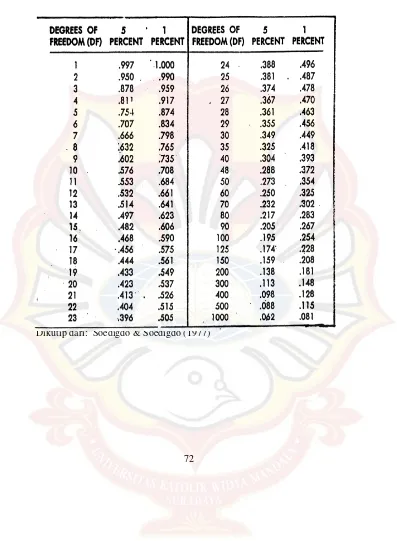
72 LAMPIRAN
TABEL UJI
Dikutip dari: Soedigdo & Soedigdo (1977) N F JI r
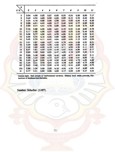
73 LAMPIRAN TABEL UJI HSD
74 LAMPIRAN H
HASIL UJI STATISTIK PERCOBAAN DAN TEORITIS SUDUT DIAM
Anova: Single Factor SUMMARY
Between Groups 0.1458 1 0.1458 0.347702 0.576931 5.987377584
Within Groups 2.51595 6 0.419325
Total 2.66175 7
7
75 LAMPIRAN I
HASIL UJI STATISTIK PERCOBAAN DAN TEORITIS KERAPUHAN GRANUL
Anova: Single Factor SUMMARY Between Groups 2.050313 1 2.050313 3.334587 0.117624 5.987377584
Within Groups 3.689175 6 0.614863
Total 5.739488 7
7
76 LAMPIRAN J
HASIL UJI STATISTIK PERCOBAAN DAN TEORITIS WAKTU LARUT
Anova: Single Factor SUMMARY
Between Groups 0.0128 1 0.0128 1.873171 0.220141 5.987377584
Within Groups 0.041 6 0.006833
Total 0.0538 7
7
77 LAMPIRAN K
HASIL UJI ANAVA SUDUT DIAM GRANUL DENGAN DESIGN-EXPERT
Use your mouse to right click on individual cells for definitions.
Response 1 Sudut diam
ANOVA for selected factorial model
Analysis of variance table [Partial sum of squares - Type III]
Sum of Mean F p-value
Source Squares df Square Value Prob > F
Model 7.54726667 3 2.515755556 7.507477 0.0103 significant
A-PVP K-30 3.16213333 1 3.162133333 9.4363871 0.0153
B-Laktosa
monohidrat 0.9075 1 0.9075 2.7081468 0.1385
AB 3.47763333 1 3.477633333 10.377897 0.0122
Pure Error 2.6808 8 0.3351
Cor Total 10.2280667 11
The Model F-value of 7.51 implies the model is significant. There is only a 1.03% chance that a "Model F-Value" this large could occur due to noise. Values of "Prob > F" less than 0.0500 indicate model terms are significant. In this case A, AB are significant model terms.
Values greater than 0.1000 indicate the model terms are not significant.
7
78
If there are many insignificant model terms (not counting those required to support hierarchy), model reduction may improve your model.
Std. Dev. 0.57887823 R-Squared 0.7378977
Mean 36.7233333 Adj R-Squared 0.6396093
C.V. % 1.57632266
Pred
R-Squared 0.4102698
PRESS 6.0318 Adeq Precision 6.2933447
The "Pred R-Squared" of 0.4103 is not as close to the "Adj R-Squared" of 0.6396 as one might normally expect. This may indicate a large block effect or a possible problem with your model and/or data. Things to consider are model reduction, response tranformation, outliers, etc. "Adeq Precision" measures the signal to noise ratio. A ratio greater than 4 is desirable. Your ratio of 6.293 indicates an adequate signal. This model can be used to navigate the design space.
7
79
Coefficient Standard 95% CI 95% CI
Factor Estimate df Error Low High VIF
Intercept 36.7233333 1 0.16710775 36.337982 37.10868449
A-PVP K-30 -0.5133333 1 0.16710775 -0.8986845 -0.127982175 1
B-Laktosa
monohidrat -0.275 1 0.16710775 -0.6603512 0.110351158 1
AB 0.53833333 1 0.16710775 0.1529822 0.923684492 1
Final Equation in Terms of Coded Factors:
Sudut diam =
36.7233333
-0.5133333 * A
-0.275 * B
0.53833333 * A * B Final Equation in Terms of Actual Factors:
Sudut diam =
36.7233333
-0.5133333 * PVP K-30
-0.275 * Laktosa monohidrat
0.53833333 * PVP K-30 * Laktosa monohidrat
7
80
The Diagnostics Case Statistics Report has been moved to the Diagnostics Node. In the Diagnostics Node, Select Case Statistics from the View Menu.
Proceed to Diagnostic Plots (the next icon in progression). Be sure to look at the:
1) Normal probability plot of the studentized residuals to check for normality of residuals. 2) Studentized residuals versus predicted values to check for constant error.
3) Externally Studentized Residuals to look for outliers, i.e., influential values. 4) Box-Cox plot for power transformations.
If all the model statistics and diagnostic plots are OK, finish up with the Model Graphs icon.
7
81 LAMPIRAN L
HASIL UJI ANAVA KERAPUHAN GRANUL DENGAN DESIGN-EXPERT
Use your mouse to right click on individual cells for definitions.
Response 2 Kerapuhan
ANOVA for selected factorial model
Analysis of variance table [Partial sum of squares - Type III]
Sum of Mean F p-value
Source Squares df Square Value Prob > F
Model 10.24333 3 3.414444444 13.98407 0.0015 significant
A-PVP K-30 2.083333 1 2.083333333 8.532423 0.0193
B-Laktosa
monohidrat 0.48 1 0.48 1.96587 0.1985
AB 7.68 1 7.68 31.45392 0.0005
Pure Error 1.953333 8 0.244166667
Cor Total 12.19667 11
The Model F-value of 13.98 implies the model is significant. There is only a 0.15% chance that a "Model F-Value" this large could occur due to noise. Values of "Prob > F" less than 0.0500 indicate model terms are significant. In this case A, AB are significant model terms.
Values greater than 0.1000 indicate the model terms are not significant.
If there are many insignificant model terms (not counting those required to support hierarchy),
8
82 model reduction may improve your model.
Std. Dev. 0.494132 R-Squared 0.839847
Mean 1.716667 Adj R-Squared 0.77979
C.V. % 28.7844 Pred R-Squared 0.639656
PRESS 4.395 Adeq Precision 8.529411
The "Pred R-Squared" of 0.6397 is in reasonable agreement with the "Adj R-Squared" of 0.7798. "Adeq Precision" measures the signal to noise ratio. A ratio greater than 4 is desirable. Your ratio of 8.529 indicates an adequate signal. This model can be used to navigate the design space.
Coefficient Standard 95% CI 95% CI
Factor Estimate df Error Low High VIF
Intercept 1.716667 1 0.14264369 1.38773 2.0456036
A-PVP K-30 -0.416667 1 0.14264369 -0.745604 -0.0877297 1
B-Laktosa
monohidrat -0.2 1 0.14264369 -0.52894 0.12893694 1
AB -0.8 1 0.14264369 -1.12894 -0.4710631 1
Final Equation in Terms of Coded Factors:
Kerapuhan =
1.716667
-0.416667 * A
8
83
-0.2 * B
-0.8 * A * B
Final Equation in Terms of Actual Factors:
Kerapuhan =
1.716667
-0.416667 * PVP K-30
-0.2 * Laktosa monohidrat
-0.8 * PVP K-30 * Laktosa monohidrat The Diagnostics Case Statistics Report has been moved to the Diagnostics Node. In the Diagnostics Node, Select Case Statistics from the View Menu.
Proceed to Diagnostic Plots (the next icon in progression). Be sure to look at the:
1) Normal probability plot of the studentized residuals to check for normality of residuals. 2) Studentized residuals versus predicted values to check for constant error.
3) Externally Studentized Residuals to look for outliers, i.e., influential values. 4) Box-Cox plot for power transformations.
If all the model statistics and diagnostic plots are OK, finish up with the Model Graphs icon.
8
84 LAMPIRAN M
HASIL UJI ANAVA WAKTU LARUT GRANUL DENGAN DESIGN-EXPERT
Use your mouse to right click on individual cells for definitions.
Response 4 Waktu larut
ANOVA for selected factorial model
Analysis of variance table [Partial sum of squares - Type III]
Sum of Mean F p-value
The Model F-value of 5.67 implies the model is significant. There is only a 2.22% chance that a "Model F-Value" this large could occur due to noise. Values of "Prob > F" less than 0.0500 indicate model terms are significant. In this case A are significant model terms.
Values greater than 0.1000 indicate the model terms are not significant.
8
85
If there are many insignificant model terms (not counting those required to support hierarchy), model reduction may improve your model.
Std. Dev. 0.08336666 R-Squared 0.68014
Mean 1.6875 Adj R-Squared 0.56019
C.V. % 4.94024652 Pred R-Squared 0.28031
PRESS 0.1251 Adeq Precision 4.29377
The "Pred R-Squared" of 0.2803 is not as close to the "Adj R-Squared" of 0.5602 as one might normally expect. This may indicate a large block effect or a possible problem with your model and/or data. Things to consider are model reduction, response tranformation, outliers, etc. "Adeq Precision" measures the signal to noise ratio. A ratio greater than 4 is desirable. Your ratio of 4.294 indicates an adequate signal. This model can be used to navigate the design space.
Coefficient Standard 95% CI 95% CI
Factor Estimate df Error Low High VIF
Intercept 1.6875 1 0.02407 1.632 1.743
A-PVP K-30 0.09916667 1 0.02407 0.04367 0.15466 1
B-Laktosa monohidrat -0.0008333 1 0.02407 -0.0563 0.05466 1
AB 0.00416667 1 0.02407 -0.0513 0.05966 1
8
86 Final Equation in Terms of Coded Factors:
Waktu larut = 1.6875 0.09916667 * A
-0.0008333 * B 0.00416667 * A * B Final Equation in Terms of Actual Factors:
Waktu larut = 1.6875
0.09916667 * PVP K-30
-0.0008333 * Laktosa monohidrat
0.00416667 * PVP K-30 * Laktosa monohidrat The Diagnostics Case Statistics Report has been moved to the Diagnostics Node. In the Diagnostics Node, Select Case Statistics from the View Menu.
Proceed to Diagnostic Plots (the next icon in progression). Be sure to look at the:
1) Normal probability plot of the studentized residuals to check for normality of residuals. 2) Studentized residuals versus predicted values to check for constant error.
3) Externally Studentized Residuals to look for outliers, i.e., influential values. 4) Box-Cox plot for power transformations.
If all the model statistics and diagnostic plots are OK, finish up with the Model Graphs icon.
8