Chapter 1
Introduction to OpenGL
Chapter Objectives
After reading this chapter, you'll be able to do the following: Appreciate in general terms what OpenGL offers
Identify different levels of rendering complexity
Understand the basic structure of an OpenGL program
Recognize OpenGL command syntax
Understand in general terms how to animate an OpenGL program This chapter introduces OpenGL. It has the following major sections:
"What Is OpenGL?" explains what OpenGL is, what it does and doesn't do, and how it works.
"A Very Simple OpenGL Program" presents a small OpenGL program and briefly discusses it. This section also defines a few basic computer-graphics terms.
"OpenGL Command Syntax" explains some of the conventions and notations used by OpenGL commands.
"OpenGL as a State Machine" describes the use of state variables in OpenGL and the commands for querying, enabling, and disabling states.
examples.
"Animation" explains in general terms how to create pictures on the screen that move, or animate.
What Is OpenGL?
OpenGL is a software interface to graphics hardware. This interface consists of about 120 distinct commands, which you use to specify the objects and operations needed to
produce interactive three-dimensional applications.
OpenGL is designed to work efficiently even if the computer that displays the graphics you create isn't the computer that runs your graphics program. This might be the case if you work in a networked computer environment where many computers are connected to one another by wires capable of carrying digital data. In this situation, the computer on which your program runs and issues OpenGL drawing commands is called the client, and the computer that receives those commands and performs the drawing is called the server. The format for transmitting OpenGL commands (called the protocol) from the client to the server is always the same, so OpenGL programs can work across a network even if the client and server are different kinds of computers. If an OpenGL program isn't
running across a network, then there's only one computer, and it is both the client and the server.
OpenGL is designed as a streamlined, hardware-independent interface to be implemented on many different hardware platforms. To achieve these qualities, no commands for performing windowing tasks or obtaining user input are included in OpenGL; instead, you must work through whatever windowing system controls the particular hardware you're using. Similarly, OpenGL doesn't provide high-level commands for describing models of three-dimensional objects. Such commands might allow you to specify relatively complicated shapes such as automobiles, parts of the body, airplanes, or molecules. With OpenGL, you must build up your desired model from a small set of geometric primitive - points, lines, and polygons. (A sophisticated library that provides these features could certainly be built on top of OpenGL - in fact, that's what Open Inventor is. See "OpenGL-related Libraries" for more information about Open Inventor.) Now that you know what OpenGL doesn't do, here's what it does do. Take a look at the color plates - they illustrate typical uses of OpenGL. They show the scene on the cover of this book, drawn by a computer (which is to say, rendered) in successively more
Figure J-1 shows the entire scene displayed as a wireframe model - that is, as if all the objects in the scene were made of wire. Each line of wire corresponds to an edge of a primitive (typically a polygon). For example, the surface of the table is constructed from triangular polygons that are positioned like slices of pie. Note that you can see portions of objects that would be obscured if the objects were solid rather than wireframe. For example, you can see the entire model of the hills outside the window even though most of this model is normally hidden by the wall of the room. The globe appears to be nearly solid because it's
composed of hundreds of colored blocks, and you see the wireframe lines for all the edges of all the blocks, even those forming the back side of the globe. The way the globe is constructed gives you an idea of how complex objects can be created by assembling lower-level objects.
Figure J-2 shows a depth-cued version of the same wireframe scene. Note that the lines farther from the eye are dimmer, just as they would be in real life, thereby giving a visual cue of depth.
Figure J-3 shows an antialiased version of the wireframe scene. Antialiasing is a technique for reducing the jagged effect created when only portions of
neighboring pixels properly belong to the image being drawn. Such jaggies are usually the most visible with near-horizontal or near-vertical lines.
Figure J-4 shows a flat-shaded version of the scene. The objects in the scene are now shown as solid objects of a single color. They appear "flat" in the sense that they don't seem to respond to the lighting conditions in the room, so they don't appear smoothly rounded.
Figure J-5 shows a lit, smooth-shaded version of the scene. Note how the scene looks much more realistic and three-dimensional when the objects are shaded to respond to the light sources in the room; the surfaces of the objects now look smoothly rounded.
Figure J-6 adds shadows and textures to the previous version of the scene. Shadows aren't an explicitly defined feature of OpenGL (there is no "shadow command"), but you can create them yourself using the techniques described in Chapter 13 . Texture mapping allows you to apply a two-dimensional texture to a three-dimensional object. In this scene, the top on the table surface is the most vibrant example of texture mapping. The walls, floor, table surface, and top (on top of the table) are all texture mapped.
Figure J-7 shows a motion-blurred object in the scene. The sphinx (or dog, depending on your Rorschach tendencies) appears to be captured as it's moving forward, leaving a blurred trace of its path of motion.
Figure J-8 shows the scene as it's drawn for the cover of the book from a different viewpoint. This plate illustrates that the image really is a snapshot of models of three-dimensional objects.
The next two color images illustrate yet more complicated visual effects that can be achieved with OpenGL:
Figure J-9 illustrates the use of atmospheric effects (collectively referred to as fog) to show the presence of particles in the air.
Figure J-10 shows the depth-of-field effect, which simulates the inability of a camera lens to maintain all objects in a photographed scene in focus. The camera focuses on a particular spot in the scene, and objects that are significantly closer or farther than that spot are somewhat blurred.
The color plates give you an idea of the kinds of things you can do with the OpenGL graphics system. The next several paragraphs briefly describe the order in which OpenGL performs the major graphics operations necessary to render an image on the screen. Appendix A, "Order of Operations" describes this order of operations in more detail.
Construct shapes from geometric primitives, thereby creating mathematical descriptions of objects. (OpenGL considers points, lines, polygons, images, and bitmaps to be primitives.)
Arrange the objects in three-dimensional space and select the desired vantage point for viewing the composed scene.
Calculate the color of all the objects. The color might be explicitly assigned by the application, determined from specified lighting conditions, or obtained by pasting a texture onto the objects.
Convert the mathematical description of objects and their associated color information to pixels on the screen. This process is called rasterization.
A Very Simple OpenGL Program
Because you can do so many things with the OpenGL graphics system, an OpenGL program can be complicated. However, the basic structure of a useful program can be simple: Its tasks are to initialize certain states that control how OpenGL renders and to specify objects to be rendered.
Before you look at an OpenGL program, let's go over a few terms. Rendering, which you've already seen used, is the process by which a computer creates images from models. These models, or objects, are constructed from geometric primitives - points, lines, and polygons - that are specified by their vertices.
The final rendered image consists of pixels drawn on the screen; a pixel - short for picture element - is the smallest visible element the display hardware can put on the screen. Information about the pixels (for instance, what color they're supposed to be) is organized in system memory into bitplanes. A bitplane is an area of memory that holds one bit of information for every pixel on the screen; the bit might indicate how red a particular pixel is supposed to be, for example. The bitplanes are themselves organized into a
framebuffer, which holds all the information that the graphics display needs to control the intensity of all the pixels on the screen.
Now look at an OpenGL program. Example 1-1 renders a white rectangle on a black background, as shown in Figure 1-1 .
Figure 1-1 : A White Rectangle on a Black Background
#include <whateverYouNeed.h>
main() {
OpenAWindowPlease();
glClearColor(0.0, 0.0, 0.0, 0.0); glClear(GL_COLOR_BUFFER_BIT); glColor3f(1.0, 1.0, 1.0);
glOrtho(-1.0, 1.0, -1.0, 1.0, -1.0, 1.0); glBegin(GL_POLYGON);
glVertex2f(-0.5, -0.5); glVertex2f(-0.5, 0.5); glVertex2f(0.5, 0.5); glVertex2f(0.5, -0.5); glEnd();
glFlush();
KeepTheWindowOnTheScreenForAWhile(); }
The first line of the main() routine opens a window on the screen: The
OpenAWindowPlease() routine is meant as a placeholder for a window system-specific routine. The next two lines are OpenGL commands that clear the window to black:
glClearColor() establishes what color the window will be cleared to, and glClear()
actually clears the window. Once the color to clear to is set, the window is cleared to that color whenever glClear() is called. The clearing color can be changed with another call to glClearColor(). Similarly, the glColor3f() command establishes what color to use for drawing objects - in this case, the color is white. All objects drawn after this point use this color, until it's changed with another call to set the color.
The next OpenGL command used in the program, glOrtho(), specifies the coordinate system OpenGL assumes as it draws the final image and how the image gets mapped to the screen. The next calls, which are bracketed by glBegin() and glEnd(), define the object to be drawn - in this example, a polygon with four vertices. The polygon's
"corners" are defined by the glVertex2f() commands. As you might be able to guess from the arguments, which are (x, y) coordinate pairs, the polygon is a rectangle.
Finally, glFlush() ensures that the drawing commands are actually executed, rather than stored in a buffer awaiting additional OpenGL commands. The
KeepTheWindowOnTheScreenForAWhile() placeholder routine forces the picture to remain on the screen instead of immediately disappearing.
OpenGL Command Syntax
constants begin with GL_, use all capital letters, and use underscores to separate words (like GL_COLOR_BUFFER_BIT).
You might also have noticed some seemingly extraneous letters appended to some command names (the 3f in glColor3f(), for example). It's true that the Color part of the command name is enough to define the command as one that sets the current color. However, more than one such command has been defined so that you can use different types of arguments. In particular, the 3 part of the suffix indicates that three arguments are given; another version of the Color command takes four arguments. The f part of the suffix indicates that the arguments are floating-point numbers. Some OpenGL commands accept as many as eight different data types for their arguments. The letters used as suffixes to specify these data types for ANSI C implementations of OpenGL are shown in Table 1-1 , along with the corresponding OpenGL type definitions. The particular
implementation of OpenGL that you're using might not follow this scheme exactly; an implementation in C++ or Ada, for example, wouldn't need to.
Table 1-1 : Command Suffixes and Argument Data Types
Suffix Data Type Typical Corresponding
C-Language Type OpenGL TypeDefinition
b 8-bit integer signed char GLbyte
s 16-bit integer short GLshort
i 32-bit integer long GLint, GLsizei
f 32-bit floating-point
float GLfloat, GLclampf
d 64-bit
floating-point double GLdouble, GLclampd
ub 8-bit unsigned integer
unsigned char GLubyte, GLboolean
us 16-bit unsigned integer
unsigned short GLushort
ui 32-bit unsigned
Thus, the two commands
glVertex2i(1, 3); glVertex2f(1.0, 3.0);
are equivalent, except that the first specifies the vertex's coordinates as 32-bit integers and the second specifies them as single-precision floating-point numbers.
Some OpenGL commands can take a final letter v, which indicates that the command takes a pointer to a vector (or array) of values rather than a series of individual arguments. Many commands have both vector and nonvector versions, but some
commands accept only individual arguments and others require that at least some of the arguments be specified as a vector. The following lines show how you might use a vector and a nonvector version of the command that sets the current color:
glColor3f(1.0, 0.0, 0.0);
float color_array[] = {1.0, 0.0, 0.0}; glColor3fv(color_array);
In the rest of this guide (except in actual code examples), OpenGL commands are
referred to by their base names only, and an asterisk is included to indicate that there may be more to the command name. For example, glColor*() stands for all variations of the command you use to set the current color. If we want to make a specific point about one version of a particular command, we include the suffix necessary to define that version. For example, glVertex*v() refers to all the vector versions of the command you use to specify vertices.
Finally, OpenGL defines the constant GLvoid; if you're programming in C, you can use this instead of void.
OpenGL as a State Machine
OpenGL is a state machine. You put it into various states (or modes) that then remain in effect until you change them. As you've already seen, the current color is a state variable. You can set the current color to white, red, or any other color, and thereafter every object is drawn with that color until you set the current color to something else. The current color is only one of many state variables that OpenGL preserves. Others control such things as the current viewing and projection transformations, line and polygon stipple patterns, polygon drawing modes, pixel-packing conventions, positions and
characteristics of lights, and material properties of the objects being drawn. Many state variables refer to modes that are enabled or disabled with the command glEnable() or
Each state variable or mode has a default value, and at any point you can query the system for each variable's current value. Typically, you use one of the four following commands to do this: glGetBooleanv(), glGetDoublev(), glGetFloatv(), or
glGetIntegerv(). Which of these commands you select depends on what data type you want the answer to be given in. Some state variables have a more specific query
command (such as glGetLight*(), glGetError(), or glGetPolygonStipple()). In addition, you can save and later restore the values of a collection of state variables on an attribute stack with the glPushAttrib() and glPopAttrib() commands. Whenever possible, you should use these commands rather than any of the query commands, since they're likely to be more efficient.
The complete list of state variables you can query is found in Appendix B . For each variable, the appendix also lists the glGet*() command that returns the variable's value, the attribute class to which it belongs, and the variable's default value.
OpenGL-related Libraries
OpenGL provides a powerful but primitive set of rendering commands, and all higher-level drawing must be done in terms of these commands. Therefore, you might want to write your own library on top of OpenGL to simplify your programming tasks. Also, you might want to write some routines that allow an OpenGL program to work easily with your windowing system. In fact, several such libraries and routines have already been written to provide specialized features, as follows. Note that the first two libraries are provided with every OpenGL implementation, the third was written for this book and is available using ftp, and the fourth is a separate product that's based on OpenGL.
The OpenGL Utility Library (GLU) contains several routines that use lower-level OpenGL commands to perform such tasks as setting up matrices for specific viewing orientations and projections, performing polygon tessellation, and rendering surfaces. This library is provided as part of your OpenGL
implementation. It's described in more detail in Appendix C and in the OpenGL Reference Manual. The more useful GLU routines are described in the chapters in this guide, where they're relevant to the topic being discussed. GLU routines use the prefix glu.
The OpenGL Extension to the X Window System (GLX) provides a means of creating an OpenGL context and associating it with a drawable window on a machine that uses the X Window System. GLX is provided as an adjunct to OpenGL. It's described in more detail in both Appendix D and the OpenGL Reference Manual. One of the GLX routines (for swapping framebuffers) is described in "Animation." GLX routines use the prefix glX.
The OpenGL Programming Guide Auxiliary Library was written specifically for this book to make programming examples simpler and yet more complete. It's the subject of the next section, and it's described in more detail in Appendix E . Auxiliary library routines use the prefix aux. "How to Obtain the Sample Code" describes how to obtain the source code for the auxiliary library.
Open Inventor is an object-oriented toolkit based on OpenGL that provides objects and methods for creating interactive three-dimensional graphics
applications. Available from Silicon Graphics and written in C++, Open Inventor provides pre-built objects and a built-in event model for user interaction, high-level application components for creating and editing three-dimensional scenes, and the ability to print objects and exchange data in other graphics formats.
The OpenGL Programming Guide Auxiliary Library
As you know, OpenGL contains rendering commands but is designed to be independent of any window system or operating system. Consequently, it contains no commands for opening windows or reading events from the keyboard or mouse. Unfortunately, it's impossible to write a complete graphics program without at least opening a window, and most interesting programs require a bit of user input or other services from the operating system or window system. In many cases, complete programs make the most interesting examples, so this book uses a small auxiliary library to simplify opening windows, detecting input, and so on.
In addition, since OpenGL's drawing commands are limited to those that generate simple geometric primitives (points, lines, and polygons), the auxiliary library includes several routines that create more complicated three-dimensional objects such as a sphere, a torus, and a teapot. This way, snapshots of program output can be interesting to look at. If you have an implementation of OpenGL and this auxiliary library on your system, the examples in this book should run without change when linked with them.
The auxiliary library is intentionally simple, and it would be difficult to build a large application on top of it. It's intended solely to support the examples in this book, but you may find it a useful starting point to begin building real applications. The rest of this section briefly describes the auxiliary library routines so that you can follow the programming examples in the rest of this book. Turn to Appendix E for more details about these routines.
Window Management
Three routines perform tasks necessary to initialize and open a window:
auxInitWindow() opens a window on the screen. It enables the Escape key to be used to exit the program, and it sets the background color for the window to black.
auxInitPosition() tells auxInitWindow() where to position a window on the screen.
auxInitDisplayMode() tells auxInitWindow() whether to create an RGBA or color-index window. You can also specify a single- or double-buffered window. (If you're working in color-index mode, you'll want to load certain colors into the color map; use auxSetOneColor() to do this.) Finally, you can use this routine to indicate that you want the window to have an associated depth, stencil, and/or accumulation buffer.
Handling Input Events
You can use these routines to register callback commands that are invoked when specified events occur.
auxReshapeFunc() indicates what action should be taken when the window is resized, moved, or exposed.
auxKeyFunc() and auxMouseFunc() allow you to link a keyboard key or a mouse button with a routine that's invoked when the key or mouse button is pressed or released.
Drawing 3-D Objects
The auxiliary library includes several routines for drawing these three-dimensional objects:
sphere octahedron cube dodecahedron torus icosahedron cylinder teapot cone
You can draw these objects as wireframes or as solid shaded objects with surface normals defined. For example, the routines for a sphere and a torus are as follows:
void auxWireSphere(GLdouble radius); void auxSolidSphere(GLdouble radius);
void auxSolidTorus(GLdouble innerRadius, GLdouble outerRadius);
All these models are drawn centered at the origin. When drawn with unit scale factors, these models fit into a box with all coordinates from -1 to 1. Use the arguments for these routines to scale the objects.
Managing a Background Process
You can specify a function that's to be executed if no other events are pending - for example, when the event loop would otherwise be idle - with auxIdleFunc(). This routine takes a pointer to the function as its only argument. Pass in zero to disable the execution of the function.
Running the Program
Within your main() routine, call auxMainLoop() and pass it the name of the routine that redraws the objects in your scene. Example 1-2 shows how you might use the auxiliary library to create the simple program shown in Example 1-1 .
Example 1-2 : A Simple OpenGL Program Using the Auxiliary Library: simple.c
#include <GL/gl.h> #include "aux.h"
int main(int argc, char** argv) {
auxInitDisplayMode (AUX_SINGLE | AUX_RGBA); auxInitPosition (0, 0, 500, 500);
auxInitWindow (argv[0]);
glClearColor (0.0, 0.0, 0.0, 0.0); glClear(GL_COLOR_BUFFER_BIT); glColor3f(1.0, 1.0, 1.0); glMatrixMode(GL_PROJECTION); glLoadIdentity();
glOrtho(-1.0, 1.0, -1.0, 1.0, -1.0, 1.0); glBegin(GL_POLYGON);
glVertex2f(-0.5, -0.5); glVertex2f(-0.5, 0.5); glVertex2f(0.5, 0.5); glVertex2f(0.5, -0.5); glEnd();
glFlush();
sleep(10); }
One of the most exciting things you can do on a graphics computer is draw pictures that move. Whether you're an engineer trying to see all sides of a mechanical part you're designing, a pilot learning to fly an airplane using a simulation, or merely a computer-game aficionado, it's clear that animation is an important part of computer graphics. In a movie theater, motion is achieved by taking a sequence of pictures (24 per second), and then projecting them at 24 per second on the screen. Each frame is moved into position behind the lens, the shutter is opened, and the frame is displayed. The shutter is momentarily closed while the film is advanced to the next frame, then that frame is displayed, and so on. Although you're watching 24 different frames each second, your brain blends them all into a smooth animation. (The old Charlie Chaplin movies were shot at 16 frames per second and are noticeably jerky.) In fact, most modern projectors display each picture twice at a rate of 48 per second to reduce flickering. Computer-graphics screens typically refresh (redraw the picture) approximately 60 to 76 times per second, and some even run at about 120 refreshes per second. Clearly, 60 per second is smoother than 30, and 120 is marginally better than 60. Refresh rates faster than 120, however, are beyond the point of diminishing returns, since the human eye is only so good.
The key idea that makes motion picture projection work is that when it is displayed, each frame is complete. Suppose you try to do computer animation of your million-frame movie with a program like this:
open_window();
If you add the time it takes for your system to clear the screen and to draw a typical frame, this program gives more and more disturbing results depending on how close to 1/24 second it takes to clear and draw. Suppose the drawing takes nearly a full 1/24 second. Items drawn first are visible for the full 1/24 second and present a solid image on the screen; items drawn toward the end are instantly cleared as the program starts on the next frame, so they present at best a ghostlike image, since for most of the 1/24 second your eye is viewing the cleared background instead of the items that were unlucky enough to be drawn last. The problem is that this program doesn't display completely drawn frames; instead, you watch the drawing as it happens.
double-buffering, every frame is shown only when the drawing is complete; the viewer never sees a partially drawn frame.
A modified version of the preceding program that does display smoothly animated graphics might look like this:
open_window_in_double_buffer_mode();
In addition to simply swapping the viewable and drawable buffers, the
swap_the_buffers() routine waits until the current screen refresh period is over so that the previous buffer is completely displayed. This routine also allows the new buffer to be completely displayed, starting from the beginning. Assuming that your system refreshes the display 60 times per second, this means that the fastest frame rate you can achieve is 60 frames per second, and if all your frames can be cleared and drawn in under 1/60 second, your animation will run smoothly at that rate.
What often happens on such a system is that the frame is too complicated to draw in 1/60 second, so each frame is displayed more than once. If, for example, it takes 1/45 second to draw a frame, you get 30 frames per second, and the graphics are idle for
1/30-1/45=1/90 second per frame. Although 1/90 second of wasted time might not sound bad, it's wasted each 1/30 second, so actually one-third of the time is wasted.
In addition, the video refresh rate is constant, which can have some unexpected
performance consequences. For example, with the 1/60 second per refresh monitor and a constant frame rate, you can run at 60 frames per second, 30 frames per second, 20 per second, 15 per second, 12 per second, and so on (60/1, 60/2, 60/3, 60/4, 60/5, ...). That means that if you're writing an application and gradually adding features (say it's a flight simulator, and you're adding ground scenery), at first each feature you add has no effect on the overall performance - you still get 60 frames per second. Then, all of a sudden, you add one new feature, and your performance is cut in half because the system can't quite draw the whole thing in 1/60 of a second, so it misses the first possible buffer-swapping time. A similar thing happens when the drawing time per frame is more than 1/30 second - the performance drops from 30 to 20 frames per second, giving a 33 percent performance hit.
Interestingly, the structure of real animation programs does not differ too much from this description. Usually, the entire buffer is redrawn from scratch for each frame, as it is easier to do this than to figure out what parts require redrawing. This is especially true with applications such as three-dimensional flight simulators where a tiny change in the plane's orientation changes the position of everything outside the window.
In most animations, the objects in a scene are simply redrawn with different
transformations - the viewpoint of the viewer moves, or a car moves down the road a bit, or an object is rotated slightly. If significant modifications to a structure are being made for each frame where there's significant recomputation, the attainable frame rate often slows down. Keep in mind, however, that the idle time after the swap_the_buffers()
routine can often be used for such calculations.
OpenGL doesn't have a swap_the_buffers() command because the feature might not be available on all hardware and, in any case, it's highly dependent on the window system. However, GLX provides such a command, for use on machines that use the X Window System:
void glXSwapBuffers(Display *dpy, Window window);
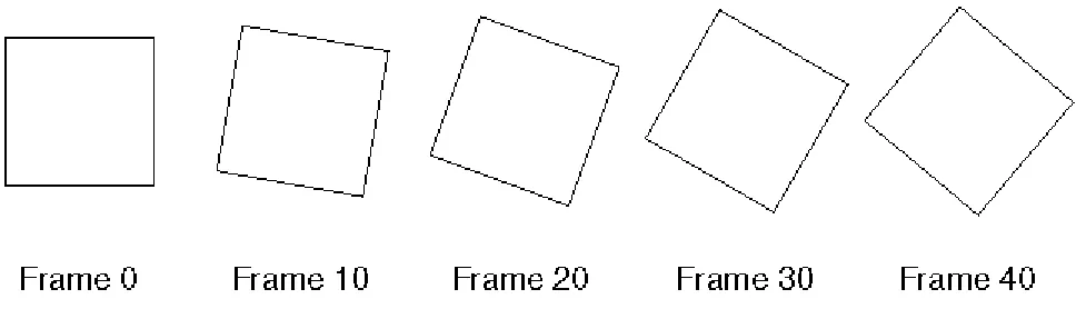
Example 1-3 illustrates the use of glXSwapBuffers() in an example that draws a square that rotates constantly, as shown in Figure 1-2 .
Figure 1-2 : A Double-Buffered Rotating Square
Example 1-3 : A Double-Buffered Program: double.c
#include <GL/gl.h> #include <GL/glu.h> #include <GL/glx.h> #include "aux.h"
static GLfloat spin = 0.0;
glClear(GL_COLOR_BUFFER_BIT);
glXSwapBuffers(auxXDisplay(), auxXWindow()); }
auxInitDisplayMode(AUX_DOUBLE | AUX_RGBA); auxInitPosition(0, 0, 500, 500);
auxReshapeFunc(myReshape); auxIdleFunc(spinDisplay);
auxMouseFunc(AUX_LEFTBUTTON, AUX_MOUSEDOWN, startIdleFunc); auxMouseFunc(AUX_MIDDLEBUTTON, AUX_MOUSEDOWN, stopIdleFunc); auxMainLoop(display);
}
[Previous chapter] [Next chapter]
Chapter 2
Drawing Geometric Objects
Chapter Objectives
After reading this chapter, you'll be able to do the following: Clear the window to an arbitrary color
Draw with any geometric primitive - points, lines, and polygons - in two or three dimensions
Control the display of those primitives - for example, draw dashed lines or outlined polygons
Specify normal vectors at appropriate points on the surface of solid objects
Force any pending drawing to complete
Although you can draw complex and interesting pictures using OpenGL, they're all constructed from a small number of primitive graphical items. This shouldn't be too surprising - look at what Leonardo da Vinci accomplished with just pencils and paintbrushes.
At the highest level of abstraction, there are three basic drawing operations: clearing the window, drawing a geometric object, and drawing a raster object. Raster objects, which include such things as two-dimensional images, bitmaps, and character fonts, are covered in Chapter 8 . In this chapter, you learn how to clear the screen and to draw geometric objects, including points, straight lines, and flat polygons.
much the same way that the globe on the cover is constructed from a large set of
rectangular blocks. The globe doesn't appear to have a smooth surface because the blocks are relatively large compared to the globe. Later in this chapter, we show you how to construct curved lines and surfaces from lots of small geometric primitives.
This chapter has the following major sections:
"A Drawing Survival Kit" explains how to clear the window and force drawing to be completed. It also gives you basic information about controlling the color of geometric objects and about hidden-surface removal.
"Describing Points, Lines, and Polygons" shows you what the set of primitive geometric objects is and how to draw them.
"Displaying Points, Lines, and Polygons" explains what control you have over the details of how primitives are drawn - for example, what diameter points have, whether lines are solid or dashed, and whether polygons are outlined or filled.
"Normal Vectors" discusses how to specify normal vectors for geometric objects and (briefly) what these vectors are for.
"Some Hints for Building Polygonal Models of Surfaces" explores the issues and techniques involved in constructing polygonal approximations to surfaces.
One thing to keep in mind as you read the rest of this chapter is that with OpenGL, unless you specify otherwise, every time you issue a drawing command, the specified object is drawn. This might seem obvious, but in some systems, you first make a list of things to draw, and when it's complete, you tell the graphics hardware to draw the items in the list. The first style is called immediate-mode graphics and is OpenGL's default style. In addition to using immediate mode, you can choose to save some commands in a list (called a display list) for later drawing. Immediate-mode graphics is typically easier to program, but display lists are often more efficient. Chapter 4 tells you how to use display lists and why you might want to use them.
A Drawing Survival Kit
Clearing the Window
Drawing on a computer screen is different from drawing on paper in that the paper starts out white, and all you have to do is draw the picture. On a computer, the memory holding the picture is usually filled with the last picture you drew, so you typically need to clear it to some background color before you start to draw the new scene. The color you use for the background depends on the application. For a word processor, you might clear to white (the color of the paper) before you begin to draw the text. If you're drawing a view from a spaceship, you clear to the black of space before beginning to draw the stars, planets, and alien spaceships. Sometimes you might not need to clear the screen at all; for example, if the image is the inside of a room, the entire graphics window gets covered as you draw all the walls.
At this point, you might be wondering why we keep talking about clearing the window - why not just draw a rectangle of the appropriate color that's large enough to cover the entire window? First, a special command to clear a window can be much more efficient than a general-purpose drawing command. In addition, as you'll see in Chapter 3 ,
OpenGL allows you to set the coordinate system, viewing position, and viewing direction arbitrarily, so it might be difficult to figure out an appropriate size and location for a window-clearing rectangle. Also, you can have OpenGL use hidden-surface removal techniques that eliminate objects obscured by others nearer to the eye; thus, if the
window-clearing rectangle is to be a background, you must make sure that it's behind all the other objects of interest. With an arbitrary coordinate system and point of view, this might be difficult. Finally, on many machines, the graphics hardware consists of multiple buffers in addition to the buffer containing colors of the pixels that are displayed. These other buffers must be cleared from time to time, and it's convenient to have a single command that can clear any combination of them. (All the possible buffers are discussed in Chapter 10 .)
As an example, these lines of code clear the window to black:
glClearColor(0.0, 0.0, 0.0, 0.0); glClear(GL_COLOR_BUFFER_BIT);
The first line sets the clearing color to black, and the next command clears the entire window to the current clearing color. The single parameter to glClear() indicates which buffers are to be cleared. In this case, the program clears only the color buffer, where the image displayed on the screen is kept. Typically, you set the clearing color once, early in your application, and then you clear the buffers as often as necessary. OpenGL keeps track of the current clearing color as a state variable rather than requiring you to specify it each time a buffer is cleared.
Chapter 5 and Chapter 10 talk about how other buffers are used. For now, all you need to know is that clearing them is simple. For example, to clear both the color buffer and the depth buffer, you would use the following sequence of commands:
glClear(GL_COLOR_BUFFER_BIT | GL_DEPTH_BUFFER_BIT);
In this case, the call to glClearColor() is the same as before, the glClearDepth()
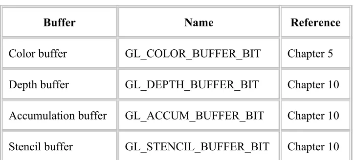
command specifies the value to which every pixel of the depth buffer is to be set, and the parameter to the glClear() command now consists of the logical OR of all the buffers to be cleared. The following summary of glClear() includes a table that lists the buffers that can be cleared, their names, and the chapter where each type of buffer is discussed.void
glClearColor(GLclampf red, GLclampf green, GLclampf blue, GLclampf alpha); Sets the current clearing color for use in clearing color buffers in RGBA mode. For more information on RGBA mode, see Chapter 5 . The red, green, blue, and alpha values are clamped if necessary to the range [0,1]. The default clearing color is (0, 0, 0, 0), which is black.
void glClear(GLbitfield mask);
Clears the specified buffers to their current clearing values. The mask argument is a bitwise-ORed combination of the values listed in Table 2-1 .
Table 2-1 : Clearing Buffers
Buffer Name Reference
Color buffer GL_COLOR_BUFFER_BIT Chapter 5
Depth buffer GL_DEPTH_BUFFER_BIT Chapter 10
Accumulation buffer GL_ACCUM_BUFFER_BIT Chapter 10
Stencil buffer GL_STENCIL_BUFFER_BIT Chapter 10
Before issuing a command to clear multiple buffers, you have to set the values to which each buffer is to be cleared if you want something other than the default color, depth value, accumulation color, and stencil index. In addition to the glClearColor() and
glClearDepth() commands that set the current values for clearing the color and depth buffers, glClearIndex(), glClearAccum(), and glClearStencil() specify the color index, accumulation color, and stencil index used to clear the corresponding buffers. See Chapter 5 and Chapter 10 for descriptions of these buffers and their uses.
graphics hardware allows sets of buffers to be cleared simultaneously. Hardware that doesn't support simultaneous clears performs them sequentially. The difference between
glClear(GL_COLOR_BUFFER_BIT | GL_DEPTH_BUFFER_BIT);
and
glClear(GL_COLOR_BUFFER_BIT); glClear(GL_DEPTH_BUFFER_BIT);
is that although both have the same final effect, the first example might run faster on many machines. It certainly won't run more slowly.
Specifying a Color
With OpenGL, the description of the shape of an object being drawn is independent of the description of its color. Whenever a particular geometric object is drawn, it's drawn using the currently specified coloring scheme. The coloring scheme might be as simple as "draw everything in fire-engine red," or might be as complicated as "assume the object is made out of blue plastic, that there's a yellow spotlight pointed in such and such a
direction, and that there's a general low-level reddish-brown light everywhere else." In general, an OpenGL programmer first sets the color or coloring scheme, and then draws the objects. Until the color or coloring scheme is changed, all objects are drawn in that color or using that coloring scheme. This method helps OpenGL achieve higher drawing performance than would result if it didn't keep track of the current color.
For example, the pseudocode
set_current_color(red); draw_object(A);
draw_object(B);
set_current_color(green); set_current_color(blue); draw_object(C);
draws objects A and B in red, and object C in blue. The command on the fourth line that sets the current color to green is wasted.
Coloring, lighting, and shading are all large topics with entire chapters or large sections devoted to them. To draw geometric primitives that can be seen, however, you need some basic knowledge of how to set the current color; this information is provided in the next paragraphs. For details on these topics, see Chapter 5 and Chapter 6 .
To set a color, use the command glColor3f(). It takes three parameters, all of which are floating-point numbers between 0.0 and 1.0. The parameters are, in order, the red, green, and blue components of the color. You can think of these three values as specifying a "mix" of colors: 0.0 means don't use any of that component, and 1.0 means use all you can of that component. Thus, the code
glColor3f(1.0, 0.0, 0.0);
gray (halfway between black and white). Here are eight commands and the colors they
You might have noticed earlier that when you're setting the color to clear the color buffer,
glClearColor() takes four parameters, the first three of which match the parameters for
glColor3f(). The fourth parameter is the alpha value; it's covered in detail in "Blending." For now, always set the fourth parameter to 0.0.
Forcing Completion of Drawing
Most modern graphics systems can be thought of as an assembly line, sometimes called a graphics pipeline. The main central processing unit (CPU) issues a drawing command, perhaps other hardware does geometric transformations, clipping occurs, then shading or texturing is performed, and finally, the values are written into the bitplanes for display (see Appendix A for details on the order of operations). In high-end architectures, each of these operations is performed by a different piece of hardware that's been designed to perform its particular task quickly. In such an architecture, there's no need for the CPU to wait for each drawing command to complete before issuing the next one. While the CPU is sending a vertex down the pipeline, the transformation hardware is working on
transforming the last one sent, the one before that is being clipped, and so on. In such a system, if the CPU waited for each command to complete before issuing the next, there could be a huge performance penalty.
In addition, the application might be running on more than one machine. For example, suppose that the main program is running elsewhere (on a machine called the client), and that you're viewing the results of the drawing on your workstation or terminal (the server), which is connected by a network to the client. In that case, it might be horribly inefficient to send each command over the network one at a time, since considerable overhead is often associated with each network transmission. Usually, the client gathers a collection of commands into a single network packet before sending it. Unfortunately, the network code on the client typically has no way of knowing that the graphics program is finished drawing a frame or scene. In the worst case, it waits forever for enough
begin execution, thereby guaranteeing that all previous commands execute in finite time even if no further rendering commands are executed.
A few commands - for example, commands that swap buffers in double-buffer mode - automatically flush pending commands onto the network before they can occur. void
glFlush(void);
Forces previously issued OpenGL commands to begin execution, thus guaranteeing that they complete in finite time.
If glFlush() isn't sufficient for you, try glFinish(). This command flushes the network as
glFlush() does and then waits for notification from the graphics hardware or network indicating that the drawing is complete in the framebuffer. You might need to use
glFinish() if you want to synchronize tasks - for example, to make sure that your three-dimensional rendering is on the screen before you use Display PostScript to draw labels on top of the rendering. Another example would be to ensure that the drawing is complete before it begins to accept user input. After you issue a glFinish() command, your
graphics process is blocked until it receives notification from the graphics hardware (or client, if you're running over a network) that the drawing is complete. Keep in mind that excessive use of glFinish() can reduce the performance of your application, especially if you're running over a network, because it requires round-trip communication. If
glFlush() is sufficient for your needs, use it instead of glFinish().void glFinish(void); Forces all previously issued OpenGL commands to complete. This command doesn't return until all effects from previous commands are fully realized.
Hidden-Surface Removal Survival Kit
When you draw a scene composed of three-dimensional objects, some of them might obscure all or parts of others. Changing your viewpoint can change the obscuring relationship. For example, if you view the scene from the opposite direction, any object that was previously in front of another is now behind it. To draw a realistic scene, these obscuring relationships must be maintained. If your code works something like this
while (1) {
get_viewing_point_from_mouse_position(); glClear(GL_COLOR_BUFFER_BIT);
draw_3d_object_A(); draw_3d_object_B(); }
it might be that for some mouse positions, object A obscures object B, and for others, the opposite relationship might hold. If nothing special is done, the preceding code always draws object B second, and thus on top of object A, no matter what viewing position is selected.
Removal," for details.) The easiest way to achieve hidden-surface removal is to use the depth buffer (sometimes called a z-buffer). (Also see Chapter 10 .)
A depth buffer works by associating a depth, or distance from the viewpoint, with each pixel on the window. Initially, the depth values for all pixels are set to the largest possible distance using the glClear() command with GL_DEPTH_BUFFER_BIT, and then the objects in the scene are drawn in any order.
Graphical calculations in hardware or software convert each surface that's drawn to a set of pixels on the window where the surface will appear if it isn't obscured by something else. In addition, the distance from the eye is computed. With depth buffering enabled, before each pixel is drawn, a comparison is done with the depth value already stored at the pixel. If the new pixel is closer to the eye than what's there, the new pixel's color and depth values replace those that are currently written into the pixel. If the new pixel's depth is greater than what's currently there, the new pixel would be obscured, and the color and depth information for the incoming pixel is discarded. Since information is discarded rather than used for drawing, hidden-surface removal can increase your performance.
To use depth buffering, you need to enable depth buffering. This has to be done only once. Each time you draw the scene, before drawing you need to clear the depth buffer and then draw the objects in the scene in any order.
To convert the preceding program fragment so that it performs hidden-surface removal, modify it to the following:
glEnable(GL_DEPTH_TEST); ...
while (1) {
glClear(GL_COLOR_BUFFER_BIT | GL_DEPTH_BUFFER_BIT); get_viewing_point_from_mouse_position();
draw_3d_object_A(); draw_3d_object_B(); }
The argument to glClear() clears both the depth and color buffers.
Describing Points, Lines, and Polygons
This section explains how to describe OpenGL geometric primitives. All geometric primitives are eventually described in terms of their vertices - coordinates that define the points themselves, the endpoints of line segments, or the corners of polygons. The next section discusses how these primitives are displayed and what control you have over their display.
You probably have a fairly good idea of what a mathematician means by the terms point, line, and polygon. The OpenGL meanings aren't quite the same, however, and it's
important to understand the differences. The differences arise because mathematicians can think in a geometrically perfect world, whereas the rest of us have to deal with real-world limitations.
For example, one difference comes from the limitations of computer-based calculations. In any OpenGL implementation, floating-point calculations are of finite precision, and they have round-off errors. Consequently, the coordinates of OpenGL points, lines, and polygons suffer from the same problems.
Another difference arises from the limitations of a bitmapped graphics display. On such a display, the smallest displayable unit is a pixel, and although pixels might be less than 1/100th of an inch wide, they are still much larger than the mathematician's infinitely small (for points) or infinitely thin (for lines). When OpenGL performs calculations, it assumes points are represented as vectors of floating-point numbers. However, a point is typically (but not always) drawn as a single pixel, and many different points with slightly different coordinates could be drawn by OpenGL on the same pixel.
Points
A point is represented by a set of floating-point numbers called a vertex. All internal calculations are done as if vertices are three-dimensional. Vertices specified by the user as two-dimensional (that is, with only x and y coordinates) are assigned a z coordinate equal to zero by OpenGL.
Advanced
OpenGL works in the homogeneous coordinates of three-dimensional projective
geometry, so for internal calculations, all vertices are represented with four floating-point coordinates (x, y, z, w). If w is different from zero, these coordinates correspond to the euclidean three-dimensional point (x/w, y/w, z/w). You can specify the w coordinate in OpenGL commands, but that's rarely done. If the w coordinate isn't specified, it's
understood to be 1.0. For more information about homogeneous coordinate systems, see Appendix G .
Lines
Figure 2-1 : Two Connected Series of Line Segments
Polygons
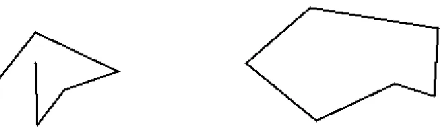
Polygons are the areas enclosed by single closed loops of line segments, where the line segments are specified by the vertices at their endpoints. Polygons are typically drawn with the pixels in the interior filled in, but you can also draw them as outlines or a set of points, as described in "Polygon Details."
Figure 2-2 : Valid and Invalid Polygons
For many applications, you need nonsimple polygons, nonconvex polygons, or polygons with holes. Since all such polygons can be formed from unions of simple convex
polygons, some routines to describe more complex objects are provided in the GLU. These routines take complex descriptions and tessellate them, or break them down into groups of the simpler OpenGL polygons that can then be rendered. (See Appendix C for more information about the tessellation routines.) The reason for OpenGL's restrictions on valid polygon types is that it's simpler to provide fast polygon-rendering hardware for that restricted class of polygons.
Since OpenGL vertices are always three-dimensional, the points forming the boundary of a particular polygon don't necessarily lie on the same plane in space. (Of course, they do in many cases - if all the z coordinates are zero, for example, or if the polygon is a triangle.) If a polygon's vertices don't lie in the same plane, then after various rotations in space, changes in the viewpoint, and projection onto the display screen, the points might no longer form a simple convex polygon. For example, imagine a four-point quadrilateral where the points are slightly out of plane, and look at it almost edge-on. You can get a nonsimple polygon that resembles a bow tie, as shown in Figure 2-3 , which isn't guaranteed to render correctly. This situation isn't all that unusual if you approximate surfaces by quadrilaterals made of points lying on the true surface. You can always avoid the problem by using triangles, since any three points always lie on a plane.
Figure 2-3 : Nonplanar Polygon Transformed to Nonsimple Polygon
Rectangles
Since rectangles are so common in graphics applications, OpenGL provides a filled-rectangle drawing primitive, glRect*(). You can draw a rectangle as a polygon, as described in "OpenGL Geometric Drawing Primitives," but your particular
implementation of OpenGL might have optimized glRect*() for rectangles.void
glRect{sifd}(TYPEx1, TYPEy1, TYPEx2, TYPEy2); void glRect{sifd}v(TYPE*v1, TYPE*v2);
function is used, the corners are given by two pointers to arrays, each of which contains an (x, y) pair.
Note that although the rectangle begins with a particular orientation in three-dimensional space (in the x-y plane and parallel to the axes), you can change this by applying rotations or other transformations. See Chapter 3 for information about how to do this.
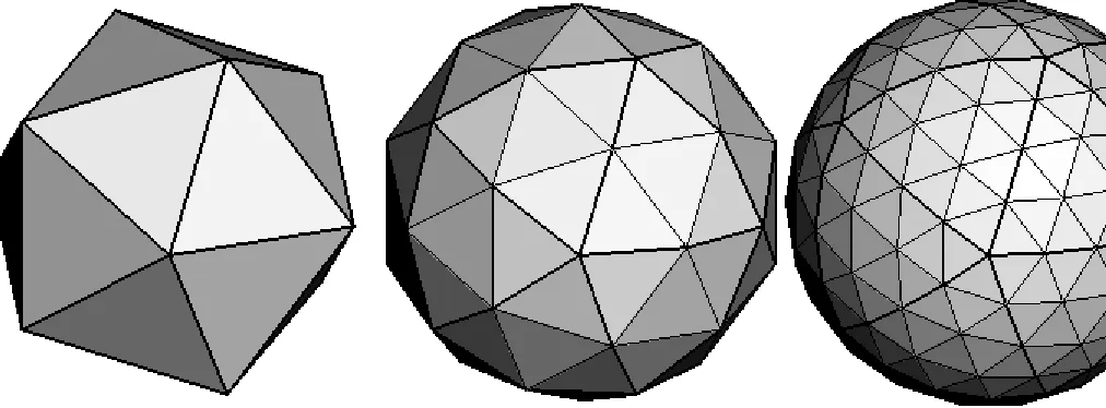
Curves
Any smoothly curved line or surface can be approximated - to any arbitrary degree of accuracy - by short line segments or small polygonal regions. Thus, subdividing curved lines and surfaces sufficiently and then approximating them with straight line segments or flat polygons makes them appear curved (see Figure 2-4 ). If you're skeptical that this really works, imagine subdividing until each line segment or polygon is so tiny that it's smaller than a pixel on the screen.
Figure 2-4 : Approximating Curves
Even though curves aren't geometric primitives, OpenGL does provide some direct support for drawing them. See Chapter 11 for information about how to draw curves and curved surfaces.
Specifying Vertices
With OpenGL, all geometric objects are ultimately described as an ordered set of vertices. You use the glVertex*() command to specify a vertex. void glVertex{234} {sifd}[v](TYPEcoords);
Specifies a vertex for use in describing a geometric object. You can supply up to four coordinates (x, y, z, w) for a particular vertex or as few as two (x, y) by selecting the appropriate version of the command. If you use a version that doesn't explicitly specify z or w, z is understood to be 0 and w is understood to be 1. Calls to glVertex*() should be executed between a glBegin() and glEnd() pair.
Here are some examples of using glVertex*():
glVertex2s(2, 3);
glVertex4f(2.3, 1.0, -2.2, 2.0);
GLdouble dvect[3] = {5.0, 9.0, 1992.0}; glVertex3dv(dvect);
The first example represents a vertex with three-dimensional coordinates (2, 3, 0). (Remember that if it isn't specified, the z coordinate is understood to be 0.) The coordinates in the second example are (0.0, 0.0, 3.1415926535898) (double-precision floating-point numbers). The third example represents the vertex with three-dimensional coordinates (1.15, 0.5, -1.1). (Remember that the x, y, and z coordinates are eventually divided by the w coordinate.) In the final example, dvect is a pointer to an array of three double-precision floating-point numbers.
On some machines, the vector form of glVertex*() is more efficient, since only a single parameter needs to be passed to the graphics subsystem, and special hardware might be able to send a whole series of coordinates in a single batch. If your machine is like this, it's to your advantage to arrange your data so that the vertex coordinates are packed sequentially in memory.
OpenGL Geometric Drawing Primitives
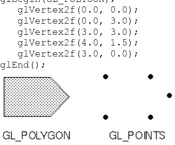
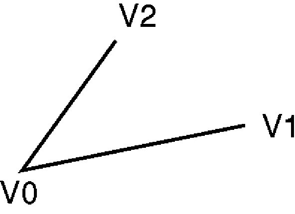
Now that you've seen how to specify vertices, you still need to know how to tell OpenGL to create a set of points, a line, or a polygon from those vertices. To do this, you bracket each set of vertices between a call to glBegin() and a call to glEnd(). The argument passed to glBegin() determines what sort of geometric primitive is constructed from the vertices. For example, the following code specifies the vertices for the polygon shown in Figure 2-5 :
glBegin(GL_POLYGON); glVertex2f(0.0, 0.0); glVertex2f(0.0, 3.0); glVertex2f(3.0, 3.0); glVertex2f(4.0, 1.5); glVertex2f(3.0, 0.0); glEnd();
Figure 2-5 : Drawing a Polygon or a Set of Points
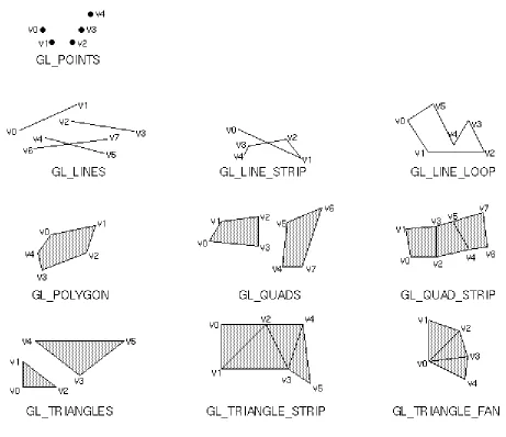
If you had used GL_POINTS instead of GL_POLYGON, the primitive would have been simply the five points shown in Figure 2-5 . Table 2-2 in the following function summary for glBegin() lists the ten possible arguments and the corresponding type of
Marks the beginning of a vertex list that describes a geometric primitive. The type of primitive is indicated by mode, which can be any of the values shown in Table 2-2 .
Table 2-2 : Geometric Primitive Names and Meanings
Value Meaning
GL_POINTS individual points
GL_LINES pairs of vertices interpreted as individual line segments
GL_POLYGON boundary of a simple, convex polygon
GL_TRIANGLES triples of vertices interpreted as triangles
GL_QUADS quadruples of vertices interpreted as four-sided polygons
GL_LINE_STRIP series of connected line segments
GL_LINE_LOOP same as above, with a segment added between last and first vertices
GL_TRIANGLE_STRIP linked strip of triangles
GL_TRIANGLE_FAN linked fan of triangles
GL_QUAD_STRIP linked strip of quadrilaterals
void glEnd(void);
Marks the end of a vertex list.
Figure 2-6 : Geometric Primitive Types
As you read the following descriptions, assume that n vertices (v0, v1, v2, ... , vn-1) are described between a glBegin() and glEnd() pair.
GL_POINTS
Draws a point at each of the n vertices. GL_LINES
Draws a series of unconnected line segments. Segments are drawn between v0 and v1, between v2 and v3, and so on. If n is odd, the last segment is drawn between 3 and vn-2, and vn-1 is ignored.
GL_POLYGON
Draws a polygon using the points v0, ... , vn-1 as vertices. n must be at least 3, or nothing is drawn. In addition, the polygon specified must not intersect itself and must be convex. If the vertices don't satisfy these conditions, the results are unpredictable.
Draws a series of triangles (three-sided polygons) using vertices v0, v1, v2, then v3, v4, v5, and so on. If n isn't an exact multiple of 3, the final one or two vertices are ignored. GL_LINE_STRIP
Draws a line segment from v0 to v1, then from v1 to v2, and so on, finally drawing the segment from vn-2 to vn-1. Thus, a total of n-1 line segments are drawn. Nothing is drawn unless n is larger than 1. There are no restrictions on the vertices describing a line strip (or a line loop); the lines can intersect arbitrarily.
GL_LINE_LOOP
Same as GL_LINE_STRIP, except that a final line segment is drawn from vn-1 to v0, completing a loop.
GL_QUADS
Draws a series of quadrilaterals (four-sided polygons) using vertices v0, v1, v2, v3, then v4, v5, v6, v7, and so on. If n isn't a multiple of 4, the final one, two, or three vertices are ignored.
GL_QUAD_STRIP
Draws a series of quadrilaterals (four-sided polygons) beginning with v0, v1, v3, v2, then v2, v3, v5, v4, then v4, v5, v7, v6, and so on. See Figure 2-6 . n must be at least 4 before anything is drawn, and if n is odd, the final vertex is ignored.
GL_TRIANGLE_STRIP
Draws a series of triangles (three-sided polygons) using vertices v0, v1, v2, then v2, v1, v3 (note the order), then v2, v3, v4, and so on. The ordering is to ensure that the triangles are all drawn with the same orientation so that the strip can correctly form part of a surface. Figure 2-6 should make the reason for the ordering obvious. n must be at least 3 for anything to be drawn.
GL_TRIANGLE_FAN
Same as GL_TRIANGLE_STRIP, except that the vertices are v0, v1, v2, then v0, v2, v3, then v0, v3, v4, and so on. Look at Figure 2-6 .
Restrictions on Using glBegin() and glEnd()
The most important information about vertices is their coordinates, which are specified by the glVertex*() command. You can also supply additional vertex-specific data for each vertex - a color, a normal vector, texture coordinates, or any combination of these - using special commands. In addition, a few other commands are valid between a
glBegin() and glEnd() pair. Table 2-3 contains a complete list of such valid commands.
Table 2-3 : Valid Commands between glBegin() and glEnd()
Command Purpose of Command Reference
glVertex*() set vertex coordinates Chapter 2
glColor*() set current color Chapter 5
glNormal*() set normal vector coordinates Chapter 2
glEvalCoord*() generate coordinates Chapter 11
glCallList(), glCallLists() execute display list(s) Chapter 4
glTexCoord*() set texture coordinates Chapter 9
glEdgeFlag*() control drawing of edges Chapter 2
glMaterial*() set material properties Chapter 6
No other OpenGL commands are valid between a glBegin() and glEnd() pair, and making any other OpenGL call generates an error. Note, however, that only OpenGL commands are restricted; you can certainly include other programming-language constructs. For example, the following code draws an outlined circle:
#define PI 3.1415926535897; GLint circle_points = 100; glBegin(GL_LINE_LOOP);
for (i = 0; i < circle_points; i++) { angle = 2*PI*i/circle_points;
glVertex2f(cos(angle), sin(angle)); }
glEnd();
This example isn't the most efficient way to draw a circle, especially if you intend to do it repeatedly. The graphics commands used are typically very fast, but this code calculates an angle and calls the sin() and cos() routines for each vertex; in addition, there's the loop overhead. If you need to draw lots of circles, calculate the coordinates of the vertices once and save them in an array, create a display list (see Chapter 4 ,) or use a GLU routine (see Appendix C .)
Unless they are being compiled into a display list, all glVertex*() commands should appear between some glBegin() and glEnd() combination. (If they appear elsewhere, they don't accomplish anything.) If they appear in a display list, they are executed only if they appear between a glBegin() and a glEnd().
glBegin(GL_POINTS);
glColor3f(0.0, 1.0, 0.0); /* green */ glColor3f(1.0, 0.0, 0.0); /* red */ glVertex(...);
glColor3f(1.0, 1.0, 0.0); /* yellow */ glColor3f(0.0, 0.0, 1.0); /* blue */ glVertex(...);
glVertex(...); glEnd();
You can use any combination of the twenty-four versions of the glVertex*() command between glBegin() and glEnd(), although in real applications all the calls in any
particular instance tend to be of the same form.
Displaying Points, Lines, and Polygons
By default, a point is drawn as a single pixel on the screen, a line is drawn solid and one pixel wide, and polygons are drawn solidly filled in. The following paragraphs discuss the details of how to change these default display modes.
Point Details
To control the size of a rendered point, use glPointSize() and supply the desired size in pixels as the argument. void glPointSize(GLfloat size);
Sets the width in pixels for rendered points; size must be greater than 0.0 and by default is 1.0.
The actual collection of pixels on the screen that are drawn for various point widths depends on whether antialiasing is enabled. (Antialiasing is a technique for smoothing points and lines as they're rendered. This topic is covered in detail in "Antialiasing." ) If antialiasing is disabled (the default), fractional widths are rounded to integer widths, and a screen-aligned square region of pixels is drawn. Thus, if the width is 1.0, the square is one pixel by one pixel; if the width is 2.0, the square is two pixels by two pixels, and so on.
With antialiasing enabled, a circular group of pixels is drawn, and the pixels on the boundaries are typically drawn at less than full intensity to give the edge a smoother appearance. In this mode, nonintegral widths aren't rounded.
Most OpenGL implementations support very large point sizes. A particular
implementation, however, might limit the size of nonantialiased points to its maximum antialiased point size, rounded to the nearest integer value. You can obtain this floating-point value by using GL_POINT_SIZE_RANGE with glGetFloatv().
With OpenGL, you can specify lines with different widths and lines that are stippled in various ways - dotted, dashed, drawn with alternating dots and dashes, and so on.
Wide Lines
void glLineWidth(GLfloat width);
Sets the width in pixels for rendered lines; width must be greater than 0.0 and by default is 1.0.
The actual rendering of lines is affected by the antialiasing mode, in the same way as for points. (See "Antialiasing." ) Without antialiasing, widths of 1, 2, and 3 draw lines one, two, and three pixels wide. With antialiasing enabled, nonintegral line widths are
possible, and pixels on the boundaries are typically partially filled. As with point sizes, a particular OpenGL implementation might limit the width of nonantialiased lines to its maximum antialiased line width, rounded to the nearest integer value. You can obtain this floating-point value by using GL_LINE_WIDTH_RANGE with glGetFloatv().
Keep in mind that by default lines are one pixel wide, so they appear wider on lower-resolution screens. For computer displays, this isn't typically an issue, but if you're using OpenGL to render to a high-resolution plotter, one-pixel lines might be nearly invisible. To obtain resolution-independent line widths, you need to take into account the physical dimensions of pixels.
Advanced
With nonantialiased wide lines, the line width isn't measured perpendicular to the line. Instead, it's measured in the y direction if the absolute value of the slope is less than 1.0; otherwise, it's measured in the x direction. The rendering of an antialiased line is exactly equivalent to the rendering of a filled rectangle of the given width, centered on the exact line. See "Polygon Details," for a discussion of the rendering of filled polygonal regions.
Stippled Lines
To make stippled (dotted or dashed) lines, you use the command glLineStipple() to define the stipple pattern, and then you enable line stippling with glEnable():
glLineStipple(1, 0x3F07); glEnable(GL_LINE_STIPPLE);
void glLineStipple(GLint factor, GLushort pattern);
stippling must be enabled by passing GL_LINE_STIPPLE to glEnable(); it's disabled by passing the same argument to glDisable().
With the preceding example and the pattern 0x3F07 (which translates to
0011111100000111 in binary), a line would be drawn with 3 pixels on, then 5 off, 6 on, and 2 off. (If this seems backward, remember that the low-order bits are used first.) If factor had been 2, the pattern would have been elongated: 6 pixels on, 10 off, 12 on, and 4 off. Figure 2-7 shows lines drawn with different patterns and repeat factors. If you don't enable line stippling, drawing proceeds as if pattern were 0xFFFF and factor 1. (Use
glDisable() with GL_LINE_STIPPLE to disable stippling.) Note that stippling can be used in combination with wide lines to produce wide stippled lines.
Figure 2-7 : Stippled Lines
One way to think of the stippling is that as the line is being drawn, the pattern is shifted by one bit each time a pixel is drawn (or factor pixels are drawn, if factor isn't 1). When a series of connected line segments is drawn between a single glBegin() and glEnd(), the pattern continues to shift as one segment turns into the next. This way, a stippling pattern continues across a series of connected line segments. When glEnd() is executed, the pattern is reset, and - if more lines are drawn before stippling is disabled - the stippling restarts at the beginning of the pattern. If you're drawing lines with GL_LINES, the pattern resets for each independent line.
Figure 2-8 : Wide Stippled Lines
Example 2-1 : Using Line Stipple Patterns: lines.c
#include <GL/gl.h> #include <GL/glu.h> #include "aux.h"
#define drawOneLine(x1,y1,x2,y2) glBegin(GL_LINES); \ glVertex2f ((x1),(y1)); glVertex2f ((x2),(y2)); glEnd();
void myinit (void) {
/* background to be cleared to black */ glClearColor (0.0, 0.0, 0.0, 0.0);
glShadeModel (GL_FLAT); }
void display(void) {
int i;
glClear (GL_COLOR_BUFFER_BIT); /* draw all lines in white */ glColor3f (1.0, 1.0, 1.0);
/* in 1st row, 3 lines, each with a different stipple */ glEnable (GL_LINE_STIPPLE);
glLineStipple (1, 0x0101); /* dotted */ drawOneLine (50.0, 125.0, 150.0, 125.0); glLineStipple (1, 0x00FF); /* dashed */ drawOneLine (150.0, 125.0, 250.0, 125.0);
glLineStipple (1, 0x1C47); /* dash/dot/dash */ drawOneLine (250.0, 125.0, 350.0, 125.0);
/* in 2nd row, 3 wide lines, each with different stipple */ glLineWidth (5.0);
glLineStipple (1, 0x0101);
drawOneLine (50.0, 100.0, 150.0, 100.0); glLineStipple (1, 0x00FF);
drawOneLine (150.0, 100.0, 250.0, 100.0); glLineStipple (1, 0x1C47);
glLineWidth (1.0);
/* in 3rd row, 6 lines, with dash/dot/dash stipple, */ /* as part of a single connected line strip */ glLineStipple (1, 0x1C47);
glBegin (GL_LINE_STRIP); for (i = 0; i < 7; i++)
auxInitDisplayMode (AUX_SINGLE | AUX_RGBA); auxInitPosition (0, 0, 400, 150);
auxInitWindow (argv[0]); myinit ();
auxMainLoop(display); }
Polygon Details
Polygons are typically drawn by filling in all the pixels enclosed within the boundary, but you can also draw them as outlined polygons, or simply as points at the vertices. A filled polygon might be solidly filled, or stippled with a certain pattern. Although the exact details are omitted here, polygons are drawn in such a way that if adjacent polygons share an edge or vertex, the pixels making up the edge or vertex are drawn exactly once - they're included in only one of the polygons. This is done so that partially transparent polygons don't have their edges drawn twice, which would make those edges appear darker (or brighter, depending on what color you're drawing with). Note that it might result in narrow polygons having no filled pixels in one or more rows or columns of pixels. Antialiasing polygons is more complicated than for points and lines; see "Antialiasing," for details.
Polygons as Points, Outlines, or Solids