DOI 10.1007/s10640-009-9321-5
Measuring the Benefits of Neighbourhood Park
Amenities: Application and Comparison of Spatial
Hedonic Approaches
Tadao Hoshino · Koichi Kuriyama
Accepted: 3 September 2009 / Published online: 23 September 2009 © Springer Science+Business Media B.V. 2009
Abstract The hedonic price method was used to estimate the influence of parks on the rental prices of single-room dwellings in Setagaya Ward, Tokyo, Japan. A simple least squares method is not optimal when the data set contains spatial autocorrelation. To improve the accuracy of estimates, we employed spatial autoregression and kriging models, resulting in a higher validity of the spatial models compared to the least squares model. Kriging models were superior to others particularly in terms of prediction accuracy, indicating that these models should be employed if the objective is superior prediction rather than estimation. The results showed that the effect of parks on property values varied with the buffer distance and park size.
Keywords Hedonic approach·Kriging·Spatial autocorrelation·Spatial regression models·Urban parks
1 Introduction
Urban parks have various purposes, including improving urban environments and provid-ing communication opportunities. The importance of urban park improvements is widely recognised by local municipalities as an important attraction to consumer decisions about where to reside. Improved computer technology and the rapid popularisation of Geographic
T. Hoshino
Department of Social Engineering, Tokyo Institute of Technology, 2-12-1 Ookayama, Meguro-ku, Tokyo 152-8550, Japan
e-mail: [email protected] K. Kuriyama (
B
)Division of Natural Resource Economics, Graduate School of Agriculture, Kyoto University, Oiwake-cho, Kitashirakawa,
Sakyo-ku, Kyoto 606-8502, Japan e-mail: [email protected]
Information Systems (GIS) have made detailed data about land use widely available. The availability of such geographical data has rapidly advanced hedonic approach studies that estimate the effect of open spaces (e.g.,Acharya and Bennett 2001;Cheshire and Sheppard 1995;Cho et al. 2006;Geoghegan 2002;Geoghegan et al. 1997;Irwin 2002;Irwin and Bockstael 2001;Lutzenhiser and Netusil 2001;Shultz and King 2001;Smith et al. 2002; Tyrvainen and Miettinen 2000). A common finding is that, on average, open spaces have positive effects on property prices, but that effects vary with the type of open space. For example, the global regression model ofCho et al.(2006) showed that moving 1,000 feet (∼300 m) closer to the nearest park increases mean house prices by 172 USD, whereas the local model revealed that the effects of proximity to parks on housing prices vary with the individual park, ranging from 662 USD to 840 USD.Geoghegan et al.(1997) found that within a 0.1- km radius, the proportion of open space positively influences land prices, but negatively impacts them within a 1- km radius, and suggested that individuals prefer more diverse land uses at a large scale.
In statistical analyses using spatial data, the importance of spatial correlations among observations of the efficiency and consistency of hedonic model estimates has been empha-sised. Spatial autocorrelation occurs when population members are related through their geo-graphic locations (Dubin 1988). Spatial correlation is far from surprising in hedonic housing models, as omitted variables are generally spatially correlated. Specifying all of the many spatial characteristics affecting a property would result in a function that is too complicated to compute. Thus, studies tend to visualise spatial aspects of the data in an empirically man-ageable form. We focused onspatial autoregression models, which are commonly used in spatial econometrics (Anselin 1988), andkriging models, which are commonly used in spa-tial statistics (Cressie 1993) and geostatistics (Wackernagel 2003). A hedonic approach using these explicit spatial regression techniques is calleda spatial hedonicapproach. Examples of empirical studies using the spatial hedonic approach to estimate the effect of environmental quality includeAcharya and Bennett(2001) on open spaces,Cho et al.(2006) on water and green spaces,Kim et al.(2003) on air quality,Kim and Goldsimth(2009) on swine pro-duction, Leggett and Bockstael (2000) on water quality, andPaterson and Boyle(2002) on visibility. All of these studies employed spatial econometric models, e.g., spatial lag models or spatial error models. To the best of our knowledge, our study was the first to use kriging models to estimate the effects of environmental quality.
Our primary objective was to measure the value ofneighbourhood parks1using a spatial hedonic approach in conjunction with a simple least squares hedonic approach and compare their validity. In Sect.2, we describe the econometric models used. Section3contains an overview of the study area and an explanation of the data used for the analysis. In Sect.4, we discuss the estimation results, and in Sect.5we present our conclusions.
2 Econometric Models
Hedonic models were developed to deal with markets for differentiated products. The dif-ferentiated product varies depending on the specific characteristics or attributes of the model (Palmquist 1999). The theoretical framework of the market for heterogeneous goods was
1In our definition, neighbourhood parks are parks in a residential neighbourhood that are available to all
originally developed byRosen(1974), who explained the price of any unit of a differenti-ated good as a function of a bundle of characteristics. Housing prices are the most common example of this application. To specify housing structure characteristics, the characteristics are grouped into structural characteristics, such as area or number of rooms, as well as loca-tional characteristics, such as transportation accessibility or environmental amenities and disamenities.
The simplest functional form used in hedonic studies is a linear regression model. IfPis a vector of observed property values atNpoints on the plane, then the linear hedonic function is
P=Xβ+ε, (1)
wherePis theN×1 vector of property prices;Xis theN×Kmatrix of regressors including the intercept term, structural variablesXswithKscharacteristics, and locational variablesXl withKlcharacteristics such that 1+Ks+Kl =K; βis theK×1 vector of the coefficients; andεis theN×1 vector of errors. The coefficients are simply estimated by OLS. However, OLS optimality inevitably fails in the presence of spatial autocorrelation. Below, we present the spatial econometric regression and the kriging models as typical solutions to the issue of spatial autocorrelation.
2.1 Spatial Autoregression Models
Two models are frequently used to represent the spatial autoregressive process: spatial error models and spatial lag models. In the former, spatial autocorrelation is considered to be caused by omitted variables, whereas in the latter, it is caused by spatial interactions (endogeneity).
2.1.1 Spatial Error Models
Although spatial autocorrelation caused by omitted spatially correlated variables does not bias OLS estimates, the estimates will be inefficient, and, most troubling, standard errors will be biased, leading to inaccurate hypothesis testing (Anselin 1988;Leggett and Bockstael 2000). This occurs because spatial autocorrelation in the error term,E(εε′)=, results in the formation of an error variance–covariance matrix with nonzero off-diagonal elements. In this situation,β should be estimated using a generalised least-squares (GLS) estimator
ˆ
βG L S = (X′−1X)−1X′−1Pfor efficiency. The empirical issue is then to estimate the elements of.
One way to obtain the structure ofdirectly is by modelling covariance as a function of the Euclidean distance between two locations. One of the most commonly used spatial process specifications is the autoregression form used in disturbances. In a general case,
P=Xβ+ε; ε=λWε+u
u∼N(0, σ2I) , withW =
w11 · · ·w1N ..
. . .. ... wN1· · ·wN N
, (2)
relationship between pairs of points that are farther apart than this distance equals zero. This concept is the same as therangein the kriging model explained below. In either case, the important point is that both definitions consider only the distance between two points and not direction,2a condition calledisotropy. Accordingly, the covariance of any two points that have the same distance between them will be the same, depending solely on distance, and the covariance converges to zero as the distance between them increases. This assumption is calledcovariance stationarity. From these assumptions,3 we defined two practical and empirically manageable weight matrices, one with a simpler, more traditional form and the other with more flexibility:
wheredi j is the distance between pointsiand j, andhis the boundary distance to be
esti-mated. The weight falls to zero when the distance betweeniandjequalshor more. These spatial weight matrices are row-normalized so that all row sums are set at 1. All unknown coefficients and parameters can be estimated using the maximum-likelihood method. The log-likelihood function is thus: concentrating onβandσ2)to obtain maximum-likelihood estimates.4
2.1.2 Spatial Lag Models
Unlike spatial error autocorrelation, spatial autocorrelation caused by spatial interactions (endogeneity) biases the OLS estimates. To represent this type of spatial process, the spatial lag model is given as:
assuming homoskedasticity in disturbances, whereρis the spatial lag parameter. Similarly, all unknown coefficients and parameters can be estimated using the maximum-likelihood method. The log-likelihood function can be written as:
L= −N
2The method to define and measure a distance must also be considered. Economic and social distance, as
well as geographical distance, may be applicable. The difference in significance between distance measures should be a future research topic.
3However, using these assumptions could be too simplistic, as roads and other components of transport
infrastructure are not radially symmetric (Cheshire and Sheppard 1995).
4When many observations are involved, use of the generalized method of moments is beneficial because
2.1.3 Specification Tests
To detect misspecification due to the spatial autocorrelation processes and to distinguish the nature of spatial autocorrelation in the error term (spatial error) and the dependent variable (spatial lag), we conducted modified Lagrange multiplier (LM) tests, which were developed byAnselin et al.(1996) and are computationally simple and robust. These tests are simple in that they are based on OLS residuals. For a detailed description of the calculation of the test statistics, refer toAnselin et al.(1996) orFlorax and Nijkamp(2003).
2.2 Kriging Models5
Kriging is a minimum mean square error statistical procedure for spatial prediction that assigns a differential weight to observations that are closer to the location of the dependent variable (Dubin et al. 1999). The prediction procedure corresponds to a spatial version of Goldberger’s best linear unbiased prediction (BLUP) method. There are several types of kriging models. To estimate hedonic price functions, a universal kriging model is employed, which is a combination of the standard multiple-linear regression and spatially correlated stochastic term to be estimated by ordinary kriging. Hence, the model assumes the presence of spatially correlated omitted variables, which correspond to the spatial error models.
Spatial weights are computed from the estimatedsemivariogramorcovariogram, and the covariogram corresponds to the variance–covariance function used to estimate. Estimating the covariogram requires several steps.
We considerεto be a spatially stochastic variable specifically tied to a particular location. Because modelling the joint distribution function ofεfor every location, point by point, is nearly impossible, some simplifying assumptions are needed to allow the application of the stationary assumption. Letxi represent the location of propertyi. Thus,S(xi)denotes the
stochastic error of the hedonic price equation for a property located atxi. If a stochastic
process issecond-order stationary, then
E[S(xi)] =µ, Cov[S(xi),S(xj)] =C(xi−xj), (7)
whereC is a covariogram. Equation (7) establishes that the first and second moments of distribution can be the same at all locations, and spatial interdependence is described solely as a function of the Euclidean distance between two points. This is a case of isotropy. The var-iance,C(0), is constant at any location. Alternatively, we can also assume that the difference between two values ofS(xi)is a stationary distribution, as follows:
E[S(xi)−S(xj)] =0, Var[S(xi)−S(xj)] =2γ (xi−xj), (8)
whereγ is called a semivariogram. This type of stationary phase is calledintrinsic station-ary. If the processSis second-order stationary, an intrinsic stationary appears to be implied. Under the second-order stationary process, the relationship between the semivariogram and the covariogram can be written as:
γ (d)= 1
2Var[S(x+d)−S(x)]
= 1
2Var[S(x+d)] + 1
2Var[S(x)] −Cov[S(x+d),S(x)]
=C(0)−C(d), (9)
5See, for example,Basu and Thibodeau(1998),Cressie(1993), andWackernagel(2003) for a more detailed
wheredis the Euclidean distance between two points. Accordingly, a covariogram can be derived from the corresponding semivariogram. We used exponential and spherical semivari-ogram models, as shown below:
whereθ indicates parameters to be estimated, withθ0 called thenugget;θ0+θ1, thesill;
andθ2, therange. The spherical semivariogram model actually reaches the specified sill,
θ0 +θ, at the specified range,θ2, which is a straightforward “cut-off” for the boundary
distance,h, in Eq. (3), whereas the exponential approaches the sill asymptotically. Notably, whend =3×θ2, the exponential semivariance reaches 95% of the sill value; this distance
is called thepractical range. The estimated parameters for the semivariogram are then used to compute the associated covariogram.
The first step of the experimental procedure was to estimate the semivariogram parameters using OLS residuals. In the second step, we computed the corresponding covariogram, which then led to.βwas estimated using the GLS estimator(X′ˆ−1X)−1X′ˆ−1P. Using the estimated GLS coefficients, the residuals can be recomputed and then used to re-estimate the new GLS estimator. This procedure was iterated until convergence.
3 Data
3.1 Urban Parks in Setagaya Ward
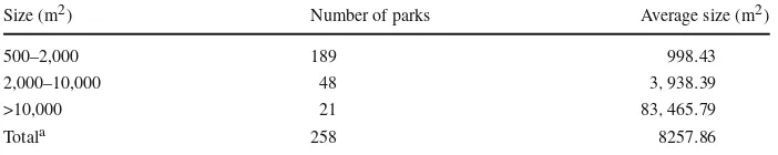
Table 1 Size classification of parks in Setagaya
Size (m2) Number of parks Average size (m2)
500–2,000 189 998.43
2,000–10,000 48 3,938.39
>10,000 21 83,465.79
Totala 258 8257.86
Source: City of Tokyo, Summary of Setagaya Ward administration, ch 7
a: River terraces, greenbelts, and parks with an area of 0–500 m2were excluded
Fig. 1 Maps of the 23 Tokyo wards and Setagaya Ward
process is quite costly. If our assumptions are not correct, our estimates may be somewhat biased. Table1summarises the size classification of parks. The number of small parks is much larger than that of large parks. Figure1shows a map of the 23 Tokyo wards, with the location of the parks used in this analysis marked in Setagaya Ward.
3.2 Data Used for Analysis
are often young, single, and/or low income) prefer neighbourhood park amenities is also important for urban housing planning.
The independent variable was the monthly rental price of a single-room dwelling, in 100-yen units (RENT). The prices and characteristics of dwellings, including AGE (age of dwelling), the log of WALK (time to walk from the nearest train station to the dwelling, in minutes), AREA (room area), and DENENd (a dummy variable, which is 1 when the nearest train station is a Denen-toshi6 line station, and 0 otherwise), were extracted in May–June 2007 from the website of Forrent, a private real-estate firm (http://www.forrent.jp). Our sample data included all single-room dwellings listed on the web page with monthly rents between 40,000 (380 USD) and 100,000 yen (950 USD). This range was set to eliminate unusually (in)expensive dwellings. The log of TAX (average tax payment of a ward inhabitant per payer population of the block), BUS-PL (number of businesses within the block area per hectare), and DAYTIMEPOP (ratio of daytime to nighttime population of the block) were created from Population Census 2006 and Setagaya Ward Statistics 2006 data. Because the inhabitant tax is pro-gressive, the TAX variable corresponds to the income level of each block. As both TAX and BUSPL increase, the rental price was also expected to increase, and as DAYTIME-POP increases, the price should decrease. Using block-level address geographical infor-mation, the Euclidean distances to Shibuya station (SHIBUYA) were calculated. Shibuya is one of the best-known districts in Japan because of its cultural and business vital-ity. Moreover, Shibuya station is an important transportation hub for anyone living in Tokyo. Thus, we inferred that as the distance to Shibuya station increases, the rental price decreases.
The Setagaya Ward Administration summary (2006) contains information on the size and location of every park in Setagaya Ward. Because the effects of park amenities on property values is not observable if the distance to the parks is too great (except for versatile large parks), we needed to define the boundary of accessible distance. A more precise estimate would require that visitors be surveyed as to their origin, means of transportation to the park, and purpose of visit. The variables for park amenities were defined as the log of PARK450 (sum of park area within a 450-m radius of the residence block midpoint), log of PARK1000 (sum of park area within a 1,000-m radius of the residence block midpoint), and LARGEPd (dummy variable, which is 1 when at least one park larger than 10,000 m2 exists within a 450-m radius of the residence block midpoint). These threshold distances were determined after extensive trials using different distances and the goodness-of-fit criterion. For the sev-eral neighbourhoods that had no parks within a 450-m radius, the value of ln PARK450 was set to 0.
3.3 Data Aggregation
Although structural characteristics were collected for all 2,370 samples, only a block-level address could be obtained for each property. To establish a one-to-one correspondence between block-level locational variables and specific dwellings, we had to aggregate each structural dwelling datum point into a block. Thus, if dwellings were highly heterogeneous even within the limited group of single-room dwellings, estimates could not be precise because some information was lost during aggregation. For the park variables, the distance
6The word denen-toshi translates to “garden city” in English, implying a desirable living environment. The
to parks was measured not from the property location, but from the block midpoint.7Using the actual distance to the nearest park as a regressor would have yielded a clearer description of the relationship between the effects of park amenities and distance to the park, but the aggregated data did not allow us to use this specification. Thus, a good hedonic approach should include datasets that are as disaggregated as possible. In-depth analysis of how data aggregation affects estimates in the context of a spatial hedonic approach will be an important topic for future research.
Additionally, heteroskedasticity often occurs when data are cross-sectionally aggregated. A traditional solution to this issue is to use the weighted least squares (WLS) method, with weights given by the number of samples in each block. Our preliminary analysis of a simple OLS model revealed that thep-value of the Breuch-Pagan test for heteroskedas-ticity was 0.092, so we decided to use the WLS method throughout our models defined in the previous section. Hence, the vector of rents P in the last section corresponds to √NiPi, . . . ,√NNPN′, whereNi indicates the number of samples belonging to blocki.
term. So, if the assumption of homoskedasticity for the vector of innovationsu in Eq. (2) and Eq. (5) holds at the individual level, the heteroskedasticity problems induced by spatial autocorrelation and by data aggregation can be solved by applying a combination of the spatial hedonic approach and the WLS method.
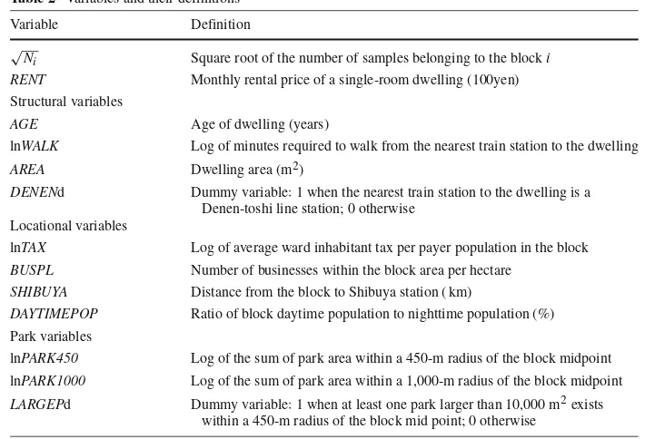
Table2lists the variables used and their definitions. Table3shows the descriptive statistics for all variables.
4 Results
Table4reports the results of the three specification tests. The spatial weight matrix used in the tests was the simple form of Eq. (3). The test of the statisticL Mλ.ρrevealed the presence
of a misspecification, with the standard WLS at 99% significance. The null hypotheses for both L Mλ andL Mρ were rejected based on the results of two one-directional tests,
indi-cating the presence of both spatial error and lag process. However, when we compared the magnitude of the statistics, L Mρ was much weaker thanL Mλwas. Thus, the main cause
of the misspecification would be the spatial autocorrelation in disturbances caused by some omitted variables. This was a positive reason to apply GLS-type estimations to the data set, including the spatial error and kriging models.
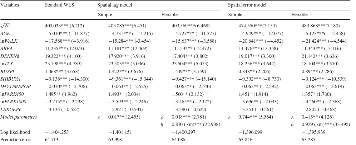
All coefficient and parameter estimation results from the five models (standard WLS, simple spatial lag, flexible spatial lag, simple spatial error, and flexible spatial error) and the two kriging models (exponential kriging, and spherical kriging) are reported in Table5and6, respectively.
7In Setagaya Ward, the largest block is 0.496 km2(1, Tamadutsumi Town), and the average block area is
Table 2 Variables and their definitions
Variable Definition
√N
i Square root of the number of samples belonging to the blocki RENT Monthly rental price of a single-room dwelling (100yen) Structural variables
AGE Age of dwelling (years)
lnWALK Log of minutes required to walk from the nearest train station to the dwelling
AREA Dwelling area (m2)
DENENd Dummy variable: 1 when the nearest train station to the dwelling is a Denen-toshi line station; 0 otherwise
Locational variables
lnTAX Log of average ward inhabitant tax per payer population in the block
BUSPL Number of businesses within the block area per hectare
SHIBUYA Distance from the block to Shibuya station ( km)
DAYTIMEPOP Ratio of block daytime population to nighttime population (%) Park variables
lnPARK450 Log of the sum of park area within a 450-m radius of the block midpoint lnPARK1000 Log of the sum of park area within a 1,000-m radius of the block midpoint
LARGEPd Dummy variable: 1 when at least one park larger than 10,000 m2exists within a 450-m radius of the block mid point; 0 otherwise
Table 3 Descriptive statisticsN=244
Variable Mean Standard deviation Min Max
√
Ni 2.857 1.247 1 7.348
RENT 712.475 59.832 530 870
√N
i×RENT 2,054.368 948.045 570.000 5,420.176
AGE 14.986 5.033 1.857 36.200
lnWALK 2.098 0.552 0.693 3.807
AREA 20.726 2.496 13.590 30.968
DENENd 0.274 0.426 0 1
lnTAX 12.391 0.432 11.513 14.618
BUSPL 5.097 5.246 0.386 56.270
DAYTIMEPOP 96.501 80.900 43.6 741.3
SHIBUYA 8.047 3.004 2.506 13.893 Park variables
lnPARK450 7.821 2.605 0 12.967
lnPARK1000 10.643 1.159 6.608 13.340
LARGEPd 0.135 0.354 0 1
Table 4 Specification tests
*** Significance at the 0.01 level
L Mλ.ρ L Mλ L Mρ
the
Benefits
o
f
N
eighbourhood
P
ark
Amenities
439
Table 5 Estimation results
Variables Standard WLS Spatial lag model Spatial error model
Simple Flexible Simple Flexible
√N
i 403.033*** (6.212) 403.085***(6.451) 403.569***(6.468) 474.550***(7.153) 483.868***(7.180)
AGE −5.010*** (−11.877) −4.731*** (−11.215) −4.727*** (−11.327) −4.949*** (−12.077) −5.123***(−12.458)
lnWALK −17.588*** (−3.916) −15.284*** (-3.454) −15.637*** (−3.588) −20.641*** (−4.452) −21.424*** (−4.544)
AREA 11.235*** (12.073) 11.181*** (12.469) 11.153*** (12.472) 11.476*** (13.358) 11.343*** (13.116)
DENENd 19.322*** (4.100) 17.920*** (3.916) 17.404*** (3.802) 19.017*** (3.300) 21.142*** (3.636)
lnTAX 23.198*** (4.789) 23.503*** (5.036) 23.504*** (5.053) 18.256*** (3.642) 18.104*** (3.570)
BUSPL 1.468*** (3.658) 1.422*** (3.676) 1.449*** (3.759) 0.848** (2.206) 0.894** (2.286)
SHIBUYA −9.136*** (−14.300) −9.361*** (−15.044) −9.427*** (−15.140) −9.392*** (−8.730) −9.124*** (−10.539)
DAYTIMEPOP −0.070*** (−2.706) −0.063** (−2.525) −0.063** (−2.540) −0.062** (−2.592) −0.063*** (−2.619)
lnPARK450 1.495** (1.962) 1.493** (2.034) 1.560** (2.132) 1.451* (1.914) 1.357* (1.780) lnPARK1000 −3.715** (−2.238) −3.593** (−2.246) −3.465** (−2.172) −3.696** (−2.033) −4.260** (−2.368)
LARGEPd −3.135 (−0.522) −2.921 (−0.504) −3.590 (−0.622) −3.351 (−0.561) −2.802 (−0.468)
Model parameters ρ 0.017** (2.455) ρ 0.018*** (2.781) λ 0.744*** (5.564) λ 0.415** (4.126)
h 0.870 ( km)*** (22.938) h 0.929 ( km)*** (33.495)
Log likelihood −1,404.253 −1,401.151 −1,400.297 −1,396.099 −1,395.939
Prediction error 64.713 63.998 64.086 63.846 63.285
Note: Dependent variable is√Ni×R E N T; structural, locational, and park variables are weighted by√Ni;N=244;t-value in parentheses
***, **, * Significance at the 0.01, 0.05, and 0.1 levels, respectively
We focus first on the overall estimation results. For structural variables, we expected RENT to be positively related to AREA and DENENd and negatively related to lnWALK and AGE. The results showed that the estimated coefficients of these variables had the expected sign at a statistically significant level. For locational variables, we expected RENT to be posi-tively related to lnTAX and BUSPL and negaposi-tively related to SHIBUYA and DAYTIME-POP. In terms of the locational variables of park amenities, we expected the basic trend to be an improvement in the residential environment as the area of parks within a buffer increased. Thus, RENT was considered to be positively related to park variables. The esti-mated coefficients of the locational variables, except for park variables, were within our predictions. The park variable results showed that lnPARK450 was significantly positive, whereas lnPARK1000 was significantly negative, and LARGEPd was insignificantly nega-tive. Interestingly,Geoghegan et al.(1997) also observed that the effects of parks vary with long and short buffers, possibly suggesting that people prefer diverse land uses at a large scale. The significance of the two log variables indicates the presence of diminishing returns for parkland. The negative effect of LARGEPd contradicts the findings of some previous studies, including that ofHidano and Takebayashi(1990), who examined the value of access to large parks in Tokyo and found that the effect of proximity to large parks on land price is positive. This discrepancy between our results might derive from the different datasets used. Since residents of single-room dwellings often do not use parks, they derive the indirect benefit of a better living environment from parks, whereas multi-room dwellers or families benefit both directly from their use of parks, as well as indirectly. We assumed that large parks often present external diseconomies, including congestion and noise, for local residents, owing to diverse applications and facilities that attract many visitors globally. Thus, especially for single-room dwellers, negative effects of large parks can cancel out their positive effects.8
Next, we compared the individual results of the seven regression models. The first area of focus was the spatial autoregression model parameters. As predicted, the results indicated that bothρandλwere significant in both the simple and flexible models; the magnitude ofρwas almost zero, whereas that ofλmaintained a certain value. Then, the likelihood ratios between the spatial error models and the standard WLS and the spatial lag model demonstrated the validity of using spatial error models.
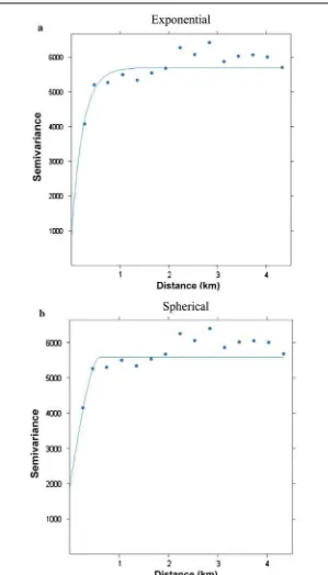
We did not find a significant difference between the spatial error models and kriging models in terms of estimated coefficient values. We could not compute the log-likelihood values of kriging models without an additional distributional assumption. Figure2a and b presents the estimated exponential and spherical semivariograms, respectively, which show a spatial interdependent relationship. Estimatedhvalues for the flexible spatial lag model and the flexible spatial error model, and thepractical rangefor the exponential model andrange for the spherical model, were 0.870, 0.929, 0.688, and 0.630 km, respectively. The kriging models detected a shorter spatial autocorrelation than did the other two models, with the boundary of spatial correlation at a 0.630–0.929- km radius, on average, from the source.9
8However, the value of large parks is not totally capitalised into local housing markets. The travel cost
method or contingent valuation method is most appropriate to evaluate such large parks. Thus, we should not underestimate the social benefits of large parks from the estimation results.
9 From the estimated boundary distance of spatial correlation (0.630–0.929 km), we may infer the spatial
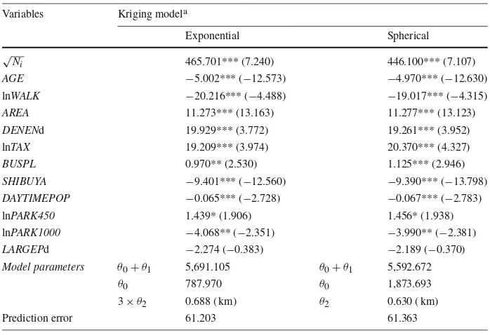
Table 6 Estimation results of the Kriging models Variables Kriging modela
Exponential Spherical
√N
i 465.701*** (7.240) 446.100*** (7.107)
AGE −5.002*** (−12.573) −4.970*** (−12.630)
lnWALK −20.216*** (−4.488) −19.017*** (−4.315)
AREA 11.273*** (13.163) 11.277*** (13.123)
DENENd 19.929*** (3.772) 19.261*** (3.952)
lnTAX 19.209*** (3.974) 20.370*** (4.327)
BUSPL 0.970** (2.530) 1.125*** (2.946)
SHIBUYA −9.401*** (−12.560) −9.390*** (−13.798)
DAYTIMEPOP −0.065*** (−2.728) −0.067*** (−2.783) lnPARK450 1.439* (1.906) 1.456* (1.938) lnPARK1000 −4.068** (−2.351) −3.990** (−2.381)
LARGEPd −2.274 (−0.383) −2.189 (−0.370)
Model parameters θ0+θ1 5,691.105 θ0+θ1 5,592.672
θ0 787.970 θ0 1,873.693
3×θ2 0.688 ( km) θ2 0.630 ( km)
Prediction error 61.203 61.363
***, **, * Significance at the 0.01, 0.05, and 0.1 levels, respectively
aTo calculatet-values of the kriging models, we used the estimated covariogram model
In all models, magnitudes of coefficients for park variables were small. When the aver-age amount of park area within a 450-m radius was evaluated, we found that an addition of a 5,000 m2park within the radius increased monthly rents of single-room dwellings only about 50 yen (0.45 USD; 1 USD = 105 JPY on 26/09/08). The addition of a 20,000-m2park within the radius increased the monthly rental price about 140 yen (1.33 USD). However, at the same time, perhaps due to the external diseconomies specific to such a large park, the overall effect was about minus 150 yen (1.43 USD) for single-room dwellings. Meanwhile at 0 parks within a 450-m radius, the addition of a 5,000-m2park within the radius increased monthly rents about 1,430 yen (13.59 USD). The addition of a 20,000-m2park within the radius increased the monthly rental price about 1,230 yen (11.69 USD). Thus, even in an area with no parks, the addition of a medium-sized park would be more beneficial than the addition of a huge park. Note that these figures should be considered a lower bound, because the data set was restricted to single-room dwellings.
4.1 Prediction Accuracy
To compare the predictive power of the models, we created a measure of prediction error. We first randomly split the samples into two subsets, with one used to estimate parameters. By using the estimated parameters, we predicted the rental price of the other subset. We then computed the absolute differences between the predicted and true values and averaged them: N P1 N P
j=1|Pj− ˆPj(θN E)|, whereNPis the total number of samples in the prediction
this analysis, we set the value ofNPto 24, which was 10% of the total sample. Thus,NE corresponds to 90% of the sample, or 220. The number of iterations was set at 300. See the last row of Table5and6. The standard WLS model had the lowest predictive power. Both the spatial lag and the spatial error models performed better than did the standard WLS model, but only slightly. No measurable differences appeared between the two specifications of spa-tial weight matrix. As expected from the nature of kriging as a spaspa-tial prediction method, the kriging models had greater predictive power than did the other models, indicating that kriging models should be employed if the objective is superior prediction rather than estimation.
5 Conclusions and Future Research
This study yielded two main empirical findings. First, the effect of neighbourhood park ame-nities on the rental price of a dwelling depends on the buffer distance and park size. Our estimation results showed that the sum of park area within a 450-m radius has a positive influence on rental prices, whereas the sum of park area within a 1,000-m radius has a neg-ative impact. Thus, individuals may prefer diverse land use at a large scale, as suggested byGeoghegan et al.(1997). For each park variable, the estimated magnitude of coefficients is small. Therefore although a particular type of park amenity is positively evaluated, other factors more directly connected to daily life, such as the availability of particular facilities, may be more important on average as a determinant of rental prices of single-room dwell-ings than parks. However, for a neighbourhood with no parks, the creation of park amenities has a measurable effect, due to the diminishing returns of parkland. Because the data set was restricted to single-room dwellings, the relatively small values are still important as a lower bound. How the effects of parks vary by dwelling type will be an interesting topic for future research. These results could help inform efficient urban planning. Our second finding was that the monthly rental prices of single-room dwellings were spatially autocorrelated, mainly due to the presence of spatially-correlated omitted variables. Consequently in terms of efficiency, spatial hedonic approaches are preferable to the basic least squares hedonic approach. In particular, in a comparison of the predictive power of the models, kriging mod-els surpassed the other modmod-els, including both spatial error modmod-els.
The most powerful use of spatial models is in finding the locational relationship between objects that can be explicitly modelled mathematically. These models can be used to predict the effects of proposed locational relationships that have not yet been implemented. Our analysis enables the comparison of current urban park planning with future proposals; our results indicate that, of the spatial models tested, kriging models will provide the best results for this objective.
Acknowledgments We want to thank Steve Gibbons, Noboru Hidano, Kenji Takeuchi, seminar participants at Osaka University and two anonymous referees for substantial ideas and helpful comments connected to the work with this paper.
References
Acharya G, Bennett LL (2001) Valuing open space and land-use patterns in urban watersheds. J Real Estate Finance Econ 22:221–237
Anselin L (1988) Spatial econometrics: methods and models. Kluwer, Dordrecht
Basu S, Thibodeau TG (1998) Analysis of spatial autocorrelation in house prices. J Real Estate Finance Econ 17:61–85
Cheshire P, Sheppard S (1995) On the price of land and the value of amenities. Economica 62:247–267 Cho SH, Bowker JM, Park WM (2006) Measuring the contribution of water and green space amenities to
housing values: an application and comparison of spatially weighted hedonic models. J Agri Resource Econ 31:485–507
City of Tokyo (2006) Setagaya Ward statistics.http://www.city.setagaya.tokyo.jp. Cited June 2007 City of Tokyo (2006) Summary of Setagaya Ward administration, ch 7.http://www.city.setagaya.tokyo.jp.
Cited May–June 2007
Cressie NA (1993) Statistics for spatial data. Wiley, New York
Dubin RA (1988) Estimation of coefficients in the presence of spatially autocorrelated error terms. Rev Econ Stat 70:466–474
Dubin RA, Pace RK, Thibodeau TG (1999) Spatial autoregression techniques for real estate data. J Real Estate Lit 7:79–95
Forrent.http://www.forrent.jp. Cited May–June 2007
Florax RJGM, Nijkamp P (2003) Misspecification in linear spatial regression models. Tinbergen Institute Discussion Paper, TI 2003-081/3
Geoghegan J (2002) The value of open spaces in residential land use. Land Use Pol 19:91–98
Geoghegan J, Wainger L, Bockstael NE (1997) Spatial landscape indices in a hedonic framework: an ecolog-ical economics analysis using GIS. Eco Econ 23:251–264
Hidano N, Takebayashi M (1990) Benefit estimation of multi-use transport facilities improvement: a hedonic approach. Infrastruct Planning Rev 8:121–128
Irwin EG (2002) The effects of open space on residential property values. Land Econ 78:465–480
Irwin EG, Bockstael NE (2001) The problem of identifying land use spillovers: measuring the effects of open space on residential property values. Am J Agri Econ 8:698–704
Kim CW, Phipps TT, Anselin L (2003) Measuring the benefits of air quality improvement: a spatial hedonic approach. J Environ Econ Manage 45:24–39
Kim J, Goldsimth P (2009) A spatial hedonic approach to asses the impact of swine production on residential property values. Environ Resource Econ 42:509–534
Kelejian HH, Prucha IR (1999) A generalized moments estimator for the autoregressive parameter in a spatial model. Int Econ Rev 40:509–533
Leggett CG, Bockstael NE (2000) Evidence of the effects of water quality on residential land prices. J Environ Econ Manage 39:121–144
Lutzenhiser M, Netusil NR (2001) The effect of open space on a home’s sale price. Contemporary Econ Pol 19:291–298
Palmquist RB (1992) Valuing localized externalities. J Urban Econ 32:40–44
Palmquist RB (1999) Hedonic models. In: Van Den Bergh JCJM (ed) Handbook of environmental and resource economics. Edward Elgar, Cheltenham, pp 765–776
Paterson WR, Boyle KJ (2002) Out of sight, out of mind? Using GIS to incorporate visibility in hedonic property value models. Land Econ 78:417–425
Rosen S (1974) Hedonic prices and implicit markets: product differentiation in pure competition. J Pol Econ 82:34–55
Shultz SD, King DA (2001) The use of census data for hedonic price estimates of open-space amenities and land use. J Real Estate Finance Econ 22:239–252
Smith V, Poulos C, Kim H (2002) Treating open space as an urban amenity. Resource Energy Econ 24:107–129 Tyrvainen L, Miettinen A (2000) Property prices and urban forest amenities. J Environ Econ Manage 39:
205–223