www.elsevier.com / locate / econbase
Finite sample properties of a QML estimator of stochastic
volatility models with long memory
a b ,
*
´
Ana Perez , Esther Ruiz
a
Department of Applied Economics(Statistics and Econometrics), Universidad de Valladolid, Valladolid, Spain b
Department of Statistics and Econometrics, Universidad Carlos III de Madrid, Madrid, Spain Received 13 December 1999; accepted 15 July 2000
Abstract
We analyse the finite sample properties of a QML estimator of LMSV models. We show up its poor performance for realistic parameter values. We discuss an identification problem when the volatility has a unit root. An empirical analysis illustrates our findings. 2001 Elsevier Science B.V. All rights reserved.
Keywords: Fractional integration; Stochastic volatility; Quasi-maximum likelihood estimator
JEL classification: C22; C15
1. Introduction
High frequency financial time series of returns are often characterised by having excess kurtosis and autocorrelated squared observations. Moreover, these autocorrelations tend to decay very slowly, suggesting that squared returns could be characterised as a long memory process; see Ding et al. (1993). This property was incorporated into Stochastic Volatility (SV) models by Harvey (1998); Breidt et al. (1998), who propose Long-Memory SV (LMSV) models and suggest estimating the parameters of these models by Quasi-Maximum Likelihood (QML) in the frequency domain. Breidt et al. (1998) prove the strong consistency of this estimator and analyse its finite sample properties for some of the parameters of the model in the stationary case concluding that the estimator behaves properly. However, the parameter values they consider in their simulations are far from the parameter values often estimated with real financial series. In this paper, we extend their study to all the parameters of the model and to a bigger range of parameter values that include more realistic and non-stationary cases and conclude that the properties of the QML estimator may be poor in some
*Corresponding author.: Tel.: 134-916-249-851; fax:134-916-249-849.
E-mail address: [email protected] (E. Ruiz).
cases of interest. Finally, we illustrate the problems faced when estimating LMSV models analysing a series of daily returns for the IBEX35 index.
2. QML estimation of LMSV models
The AutoRegressive Long Memory Stochastic Volatility (ARLMSV) model is given by:
yt5s s ´* t t (1a)
d 2
(12fL )(12L ) log (st)5ht (1b)
where st denotes the volatility of series y ,t s* is a scale parameter, ´t is a Gaussian white noise
2
process with unit variance,ht is NID(0, sh) and independent of ´t, and d can be non-integer. Model (1a,b) encompasses several SV models previously proposed in the literature. When f50, model (1a,b) becomes the basic LMSV model in Harvey (1998); if d50 and ufu,1, we obtain the ARSV (AutoRegressive SV) model in Harvey et al. (1994); when hd50, f51j or hf50, d51j, model (1a,b) becomes the RWSV (Random Walk SV) model. Notice that in the last case, the parameters of the ARLMSV model are not identified.
Model (1a,b) can be linearised as follows:
2 2
log( y )t 5m1log(st)1jt, (2)
2 2 2 2
where m5log(s*)1E(log(´t)) and jt5log(´t)2E(log(´t)). The QML estimator proposed by Harvey (1998) and Breidt et al. (1998) is obtained by maximising the discrete Whittle approximation
2
to the likelihood function of log( y ) in the frequency domain, treatingt jtas if it were Gaussian. When
20.5,d,0.5 andufu,1, the model is stationary and the QML estimator is consistent; see Breidt et al. (1998). The asymptotic distribution of QML estimators for LMSV models is still unknown. If 0.5#d#1, the model is not stationary, but taking first differences in Eq. (2) yields a stationary series
2
and QML estimation can then be carried out for D log( y ).t
Once the parameters of the model have been estimated, the underlying volatility at time t may be
˜
ˆ ˆ
estimated by s*exph0.5ht / Tj, where s* is the sample standard deviation of the heteroscedasticity
˜
corrected observations, as suggested by Harvey and Shephard (1993), and ht / T is the smoothed estimated log-volatility series obtained using the algorithm in Harvey (1998).
3. Finite sample properties of QML estimator
In this section, we analyse the finite sample properties of the Whittle estimator of the parameters of the ARLMSV model by means of several Monte Carlo experiments. As´t is assumed to be Gaussian,
2
the variance of jt is known to be p / 2 and is not estimated. For each model design and sample size considered, T51024, T54096 and T58192, we generate 3000 replicates. Table 1 displays the bias and standard deviations for some selected ARLMSV models.
In the basic stationary LMSV models (f50,d,0.5), we observe that the QML estimator of d has a
2
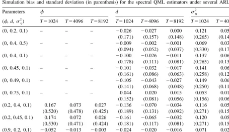
Table 1
Simulation bias and standard deviation (in parenthesis) for the spectral QML estimators under several ARLMSV models
2 (0.2, 0.4, 0.1) 0.167 0.073 0.027 20.136 20.070 20.034 0.116 0.057 0.041
(0.520) (0.478) (0.425) (0.189) (0.131) (0.092) (0.271) (0.156) (0.121) (0.2, 0.45, 0.1) 0.174 0.072 0.026 20.161 20.065 20.032 0.120 0.059 0.044
(0.530) (0.471) (0.424) (0.181) (0.117) (0.081) (0.271) (0.155) (0.123) (0.9, 0.2, 0.1) 20.052 20.013 20.003 20.024 20.020 20.016 0.071 0.024 0.013
(0.190) (0.089) (0.050) (0.171) (0.122) (0.088) (0.177) (0.071) (0.041) (0.99, 0.2, 0.1) 20.022 20.018 20.018 0.224 0.275 0.286 20.065 20.087 20.090
(0.019) (0.010) (0.007) (0.139) (0.070) (0.049) (0.052) (0.018) (0.013)
positively biased. Regarding the non-stationary model with d50.75, it seems that the QML estimator behaves better than in the stationary cases, with small standard deviations and smaller, but positive,
2
ˆ ˆ
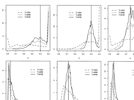
bias for d and smaller bias for sh. Fig. 1 represents kernel estimates of the simulated probability
2 2 2
densities of the QML estimates of d and sh for models with hd50.4, sh50.1j, hd50.4, sh50.5j
2
and hd50.75, sh50.1j. For the first two models, the QML estimators are not adequate at all when
ˆ
T51024. The distribution of d has always a concentration of mass at d50.5 and the situation
2
becomes not much better, even with T58192, whensh50.1. For this model, we also observe that the
2 2
ˆ ˆ
sample distribution of sh is shifted towards zero, so that we will estimate sh¯0 with high
2
probability. The estimation only improves considerably with the sample size whensh50.5, that is a value clearly bigger than the values often estimated with real data. Regarding the LMSV model with
d50.75, the empirical distributions are such that inference is reliable, even when T54096.
ˆ
In the ARLMSV models (0,d,0.5, ufu,1), there is always a negative bias in d and a positive
2
ˆ
bias insh, both decreasing the bigger is T, except for the model with f50.99. In this case, the bias
2
ˆ ˆ
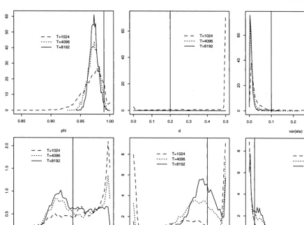
of d is positive and quite large and the bias of sh is negative, and none of them decreases with T. When the parameter d is near the boundary of non-stationarity (d50.5), the parameter f is largely overestimated and has much dispersion, while d is always underestimated. It seems that the QML estimator cannot distinguish whether the non-stationarity comes from the autoregressive polynomial (f51) or from the fractional integration (d50.5). This could be expected as the parameters of the ARLMSV model are not identified when the volatility process has a unit root. Fig. 2 displays the
2 2
2
Fig. 1. Estimated densities of spectral QML estimators of d (top panels), andsh(bottom panels) for three LMSV models, left to right:
2 2 2
hd50.4,s 5h 0.1j,hd50.4,s 5h 0.5j,hd50.75,s 5h 0.1j. Vertical line drawn on each graph indicates the true parameter value.
f50.99, none of the parameters of the ARLMSV model can be estimated with enough precision.
ˆ
When d50.4, the distribution of f has a concentration of mass close to one greater than expected, explaining the positive and large bias reported in Table 1.
Therefore, the finite sample properties of the QML estimator are such that inference on the parameters of ARLMSV models based on it may not be reliable. This conclusion contradicts the
2
results in Breidt et al. (1998). However, they only considersh51 and d5h0.2, 0.4j, where the QML estimator behaves quite well.
4. Empirical analysis of IBEX35
2
Fig. 2. Estimated densities of spectral QML estimators of f (left), d (center) and sh (right) for ARLMSV models with parameters
2 2
hf 50.99, d50.2,s 5h 0.1j(top panels) andhf 50.2, d50.4,s 5h 0.1j(bottom panels). Vertical line drawn on each graph indicates the true parameter value.
Fig. 4. Sample autocorrelations of squared returns (left) and log-squared returns (right) of IBEX35.
significant autocorrelations, even for very high lags, with a very slow decay, especially remarkable in the log-squared returns; see Fig. 4.
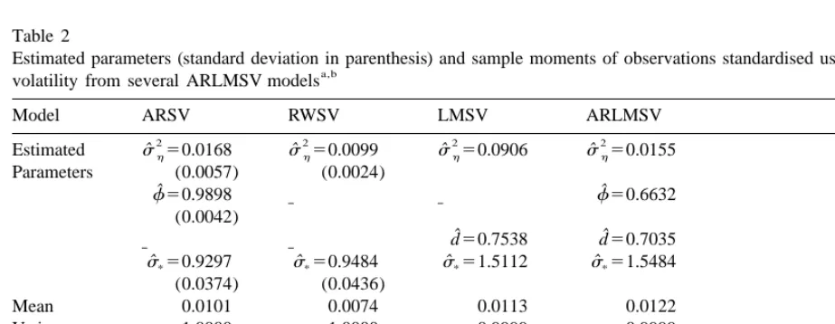
Consequently, we have first estimated the ARSV model by the QML method of Harvey et al. (1994). The estimated parameters together with their standard deviations, computed using the formulae in Ruiz (1994) and Harvey and Shephard (1993), appear in Table 2. As expected, the autoregressive parameter is estimated very close to one. The results of fitting a RWSV model are also reported in Table 2.
Regarding long memory models, we have first fitted a LMSV model, obtaining an estimate of d on
Table 2
Estimated parameters (standard deviation in parenthesis) and sample moments of observations standardised using smoothed a,b
Skewness 20.0284 20.0441 20.0183 20.0127
Kurtosis 3.5620 3.7070 3.3941 3.4380
Q (10)2 43.15 80.06 17.89 15.50
Q (50)2 101.70 144.61 71.37 68.43
Q (100)2 150.41 198.87 117.67 113.39 a
Q (k) denotes the Ljung–Box statistic for the first k autocorrelations in the squared observations.2
b
ˆ
the boundary of non-stationarity (d50.5). As Harvey (1998) suggests this could be indicating that a non-stationary model is preferable, so a model with d.0.5 has been estimated. Finally, we have also fitted an ARLMSV model. The results appear in Table 2.
Several sample moments of the standardised observations from the models previously estimated are also displayed in Table 2. The fit from long memory models is better than from the other models, with correlations in the squares being no longer significant at the 1% level. However, looking at the diagnostics on the residuals, it is difficult to distinguish between both long memory models. Notice that the implications of both models in terms of forecasting future volatilities are different because the variance of the unpredictable component in the LMSV model is bigger than in the ARLMSV model, which has an AR component that could be predicted.
In order to choose between both long memory models, and given that the asymptotic distribution of the QML estimators for these models is still unknown, we have carried out a likelihood ratio test to gauge the significance of the AR component. Recall that the ARLMSV model nests the basic LMSV
ˆ ˆ
model (f50). The value of the test statistic is LR52[log L(c)2log L(c0)]51.0885, which does
2
clearly not reject the null compared to the x1 distribution. Therefore, the LMSV model seems to be preferable.
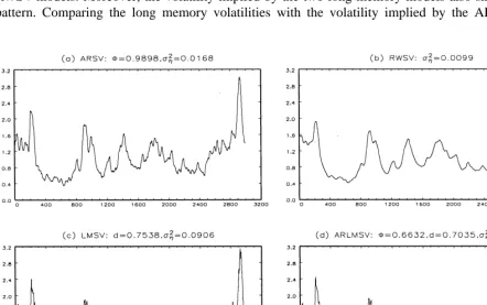
In Fig. 5, we plot the implied smoothed volatility of the IBEX35 returns for the four estimated models. As expected there is no difference between the volatilities estimated by the ARSV and the RWSV models. Moreover, the volatility implied by the two long memory models also show the same pattern. Comparing the long memory volatilities with the volatility implied by the ARSV and the
RWSV models, it is possible to observe that the fit of the former is better, especially in the high volatility periods.
5. Conclusions
We have shown that the finite sample properties of the spectral QML estimator for ARLMSV models are poor when the volatility evolves smoothly over time and / or is close to be non-stationary. Even worse, in the unit root case, the parameters of the ARLMSV model are not identified so inference is not reliable at all. When modelling the volatility of the IBEX35 index, it seems that this can be represented by a long memory process but it is difficult to establish the adequate specification of that process.
Acknowledgements
´
This research was started while Ana Perez was a visitor at the Department of Statistics and Econometrics (Universidad Carlos III de Madrid). She thanks the department for its hospitality. We are very grateful to A.C. Harvey, J. Hidalgo, F. Marmol, F. Sowell, C. Velasco, and the participants at the 1999 Time Series Workshop held in Arrabida, Portugal, specially to B. Ray and N. Crato, for helpful comments and suggestions. We also acknowledge financial support from projects SEC97-1379 and PB95-0299 by the Spanish Government. Any remaining errors are our own.
References
Breidt, F.J., Crato, N., de Lima, P.J.F., 1998. The detection and estimation of long-memory in stochastic volatility. Journal of Econometrics 83, 325–348.
Ding, Z., Granger, C.W.J., Engle, R.F., 1993. A long memory property of stock market returns and a new model. Journal of Empirical Finance 1, 83–106.
Harvey, A.C., 1998. Long memory in stochastic volatility. In: Knight, J., Satchell, E. (Eds.), Forecasting Volatility in Financial Markets. Butterworth–Haineman, London, pp. 307–320.
Harvey, A.C., Ruiz, E., Shephard, N.G., 1994. Multivariate stochastic variance models. Review of Economic Studies 61, 247–264.
Harvey, A.C., Shephard, N.G., 1993. Estimation and testing of stochastic volatility models. STICERD Econometrics Discussion Paper EM / 93 / 268, London School of Economics.