SPECTRUM-BASED OBJECT DETECTION AND TRACKING TECHNIQUE FOR
DIGITAL VIDEO SURVEILLANCE
Boris Vishnyakov, Yury Vizilter and Vladimir Knyaz
The Federal State Unitary Enterprise “State Research Institute of Aviation Systems” Moscow, Viktorenko 7, Russia
[email protected], [email protected], [email protected] http://gosniias.ru
Commission III/4: Complex Scene Analysis and 3D Reconstruction; III/5: Image Sequence Analysis
KEY WORDS:object, detection, tracking, monitoring, video, image
ABSTRACT:
This paper presents a motion detection and object tracking technique for digital video surveillance applications. Motion analysis algo-rithms are based on processing of multiple-regression pseudospectrums. Complete object detection and tracking scheme is described. Results of testing on public PETS and ETISEO test beds are outlined.
1 INTRODUCTION
The video surveillance is one of the key technologies of modern security systems. Digital video surveillance presumes the visual control of some territory with one or more video cameras, that allows storing and viewing digital video data, continuously eval-uating the state of controlled region and detecting some changes in observed scene as “security events”.
The main drawback of traditional video surveillance systems pro-viding raw video to a human operator is a serious decreasing of operator’s response capability, while the system is growing in size. This problem is especially urgent in case of city-level surveillance systems. Well-known business case is an implemen-tation of video surveillance system in London, Great Britain in-cluding tens of thousands of cameras in a single network and more than half a million cameras in the whole city. Unfortu-nately, it did not provide a serious reduction of crime incidents or increasing of crime detection rate. Now we know that it is not enough just to broadcast cameras’ video to the surveillance cen-ter. Video should be processed and alarms should be generated in real-time to attract the attention of operator in critical situations.
So, the design of high-performance intellectual video analytic systems is a very actual practical task. Moreover, such intelli-gent systems can address both security and counterterrorism ob-jectives, and can be of use in some business applications. For example, they can collect statistical information about the atten-dance of observed object, distribution of visitors over time, main routes of movement, etc. Other possible application is a traffic monitoring and so on.
The Motion analysis is a basis of all intelligent video surveillance technologies. In particular, it provides the fundamentals for au-tomatic detection and tracking of moving objects and auau-tomatic detection of new or disappeared objects of observed scene. It is the well-studied area of computer vision including many differ-ent techniques. The brief overview of these techniques is given in next section.
This paper contains a description of proposed technique accom-panied with testing results on PETS (PETS video database, n.d.) and ETISEO (ETISEO video database, n.d.) public video test beds.
2 RELATED WORKS
The motion detection and tracking problem is widely studied all around the world. There are lots of methods and algorithms, that detect motion and trace moving objects. Let us dwell on main approaches in video analysis task. First one is the optical flow approach (Horn and Schunck, 1981, Nagel, 1983, Barron et al., 1994). It was the first mentioned in (Horn and Schunck, 1981). This approach is based on finding the pixel speed from previous to current frames. LetI(k)be an input image pixel matrix with widthwand heighthon frame numberk. It is assumed that the brightness of a point remains constant during a short period of time, which is expressed by the equation
dI(k)x,y
dk = 0.
Hence we get an equation
∇I(k)x,y·(u, v)T+
∂I(k)x,y
∂k = 0,
where(u, v)T– vector of pixel movement.
Hence optical flow speed(u, v)Tcan be found via iteration method from (Horn and Schunck, 1981, Barron et al., 1994). In different books and papers the number of required iterations varies, but to achieve a good result you have to make over 100 iterations over full image, what is very time consuming.
The optical flow approach is useless if image sequence contains large amount of pixel noise. The next correlation approach (Anan-dan, 1989, Singh, 1992) is based on computing correlation func-tion of some area and minimizing it in surrounding region to find the best match for it and speed vector(u, v)T. Most of correla-tion algorithms are based on minimizacorrela-tion of SSD-funccorrela-tion (Sum of Squares Difference):
SSDk(x, y, u, v) =
=
i=n
X
i=−n j=n
X
j=−n
Wi,j(Ix+u+i,y+v+i(k+ 1)−Ix+i,y+i(k)),
being obtained more accurate on each level. In (Singh, 1992) minimum of SSD-function is found through iteration process.
But correlation approach is not robust too because it strongly de-pends on invariability of scene brightness. In (Heeger, 1988) fre-quency approach is proposed. This approach is based on “power” function, evaluated as the Gabor filter (Gabor, 1946) with fre-quenciesLx, Ly, ω:
Speed vector(u, v)Tis found during minimization of function
f(u, v) =
predicted power value,miandRiare average power values.
3 REGRESSION PSEUDOSPECTRUMS
In this section we introduce the notion of multiple-regression pseudospectrums.
Let againI(k)be an input image pixel matrix with widthwand heighthon frame numberk,I(k)∈ IRw×h
. It is assumed that I(k) is a grayscale image, so 0 ≤ I(k)x,y ≤ 255 ∀x =
1. . . w, y = 1. . . h. Let us callMn(k)an regression
accu-mulator ofnframes with parameterα, calculated on framek. It will be a matrixMn(k)∈IRw
×h
(Box et al., 1994):
Mn(k+ 1) =αMn(k) + (1−α)I(k). (1)
You can calculate the accumulator valueMn(k)on framekby
adding each older member in series (1):
Mn(k) = (1−α) k−1
X
i=0
αk−1−iI(i). (2)
Let us assume thatl(k)is an element of the image matrixI(k) andmn(k)is an element of the accumulator matrixMn(k)with
the same coordinates, asl(k). Let us suppose that on an initially zero input of accumulator (2) since some momentk0 (without
loss of generality, letk0 = 0), during enough long time some
signal with intensitylis being given:
mn(k) =l(1−α) k−1
X
i=0
αk−1−i=l(1−αk). (3)
Now it’s quite simple to find suchα, so thatmn(k)would surely
exceedβshare of signallafternframes:
mn(n) =l(1−αn) =βl.
Givenαncan be found as (4), the whole accumulator sum in one
pixel at variable framekcan be found as
mn(k) =l(1−αkn) =l 1−(1−β)k/n
. (5)
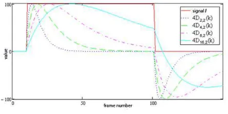
Themn(k)graphs for differentαn, n = 4,8,16,32values are
shown in Figure 1, supposedβ= 0.5, l= 100, k0= 10.
Figure 1: Accumulated pixelmn(k)for differentαn.
Thus, time averaging parameterαn, defined in (4), is in fact the
satiety parameter of the filter response function. It allows to judge after which time (in frames)naccumulated sum will be equal to βl.
According to (5),αnpossesses the multiplicity property:
αn=αsn·s. (6)
a difference between the responses of accumulators with multi-ple smoothing parameternandn·s. By (6) and assuming that some signal with intensitylis being given from timek0= 0, this
difference will possess a very interesting property:
Dn,s(n·s) =mn(n·s)−mn·s(n·s) = (7)
Consider the behaviour of derivativesDn,s(k)function. Lets=
2andβ= 0.5. Then, according to (7), difference between accu-mulator with memory of2nframes and accumulator with mem-ory ofnframes will be equal to
Dn,2(2n) = 0.25l. (8)
Figure 2 shows differencesDn,sbetween accumulators with
Figure 2: Pseudospectrum: accumulator derivativesDn,s(k).
As you can see, quadruplicate difference of multiple accumula-tors4·Dn,2(k)is a partially convex function on the segment of
the signal presence. This maximum is single and equal tol, more-over, it is reached on the frame with number2n(if this maximum can be reached at all).
Thus, first order regression derivatives behaviour with multiple memory length recalls spectral decomposition, or rather signal wavelet transformation. Let us call a multiple-regression pseu-dospectrum – set of differences of first-order regressive accumu-lators (7) with multiple characteristics of memory length by a sequence of powers of two: 1,2,4,8, . . .(view Figure 2). This pseudospectrum allows to qualitatively and quantitatively investi-gate both the duration and amplitude of the input time signal such as ”meander.”
If the maximum of differences between the responses has been consistently achieved for all accumulators with memory length N, but for accumulator with memory lengthn=N+1predicted signal maximum was not reached, it means that a constant input signal had a length of2N frames, and then began to decrease or was otherwise dramatically changed.
Similarly, we can make conclusions about the magnitude of the signal. CauseDn,2(2n) = 0.25l, for allnwhose maximum was
reached,
l= 4Dn,2(2n). (9)
Expected maximum value ofDn,2(k)can be easily found, for
example, forn = 1. Further it should be compared with the value of differences between accumulatorsDn,2(k)for othern
until maximum on framek = 2mwill be less than all previous maximums forn < m.
Now consider the problem of determining the sensitivity thresh-old of the algorithm, detecting the changes of brightness in im-ages. Figure 3 shows the shape of multiple-regression pseudospec-trum for the case of shorter time of signal presence on the image sequence.
Apparently, for lesser duration of the signal, lower frequency components of pseudospectrum start to move in the negative di-rection from higher initial values (after a reaction to the passage of the front edge of the signal) and thus achieve the appropriate extremum (in this case it will be minimum) at values lower in magnitude than the specified threshold, based on the expected drop estimate (8). Figure 3 illustrates it well by the function D16,2(k)(the lowest frequency component of the presented
pseu-dospectrum). However, this problem can be solved if we jointly consider a pair of consecutive pseudospectrum components.
Consider previousD8,2(k)toD16,2(k)pseudospectrum
compo-nent on Figure 3. Since its response to input signal change is
Figure 3: Dynamic brightness threshold correction based on pseudospectrum.
much faster, it crosses the zero line much earlier, according to signal disappearance. At this point, the value of currentD16,2(k)
component still significantly greater than zero. This value (the value of theD16,2(k)pseudospectrum component when
preced-ing componentD8,2(k)crosses zero line) is proposed to
mem-orize for each pixel and then to use in dynamic corrections to the threshold that detects brightness changes. As shown in Fig-ure 3, detection of the back front of the signal with the threshold with dynamic correction is successful even in case of significantly short, compared with the characteristic time of accumulation of this pseudospectrum component, input signal.
Analysis of the introduced multiple-regression pseudospectrums is particularly useful in the case of image analysis that studies moving objects or left/missing items. Since, on the one hand, the object’s motion relative to the background due to the effect of image pixels obstruction generates in each individual pixel tem-poral ”meander” signal, which has clearly defined leading and trailing edges (brightness fluctuations over time). On the other hand, the possibility of signal analysis based on the difference between the accumulators with multiple memory lets you signifi-cantly decrease processing time of machine vision systems. Since estimates of the time signal characteristics must be obtained in-dependently for each image pixel, in the case of using more com-plex statistics than the accumulated sums, the necessity to cal-culate the corresponding parameters estimates of the time signal directly leads to a huge increase of either computation time, or use of the program memory, or both.
4 ALGORITHMIC SCHEME
In this section we introduce the algorithmic scheme, which in-cludes image preprocessing, motion detection and object track-ing.
Objects detection and tracking are implemented as a modular three-stage procedure:
1. Detection of moving pixel groups based on pseudospectrum analysis.
2. Forming of object hypotheses and interframe object track-ing.
3. Spatiotemporal filtration of object motion parameters.
Let us consider first and second stages of this procedure.
• If signal exits in some pixels, then|Dn,2(k)|in them will
be greater than zero. It can be or a signal from the object, or some noise on the image sequence. To make an algorithm more robust, we should filter the noise with some threshold. This threshold can be found adaptively on each frame using methods described above.
• Divide the whole accumulator image on many square parts using grid. Assume each small square as moving if its value is greater than threshold and not moving (background) oth-erwise. Let us call these small image squares moving image elementsω1. . . ωm.
Moving object is created from moving image elementsω1. . . ωm.
Various moving elements exist for all values ofn(or don’t exist if there’s no moving objects on video sequence on current frame). It’s obvious that pseudospectrums with longer memory are more robust to noise, but it takes longer to react for them, when a sig-nal in some pixels starts being received. Pseudospectrums with shorter memory react to a pixel signal much faster, but they react to noise as well as to a real signal. So if an element is a moving one, its signal should exist on most of faster pseudospectrums. And if it is a new or disappeared object, its signal should ex-ist on most of slower pseudospectrums. Let us suppose that we have a set of moving objectsΛ1. . .Λs1 and set of new or
dis-appeared objects∆1. . .∆s2on a previous frame, set of moving
image elementsω1. . . ωm1and elements that concern to new or
disappeared objectsω1. . . ωm2 on current frame. So we must
somehow associate all objects with their new regions. Let us see hypotheses forming for moving objects:
• No object associates with the moving element. So this mov-ing element belongs to a new object.
• No moving element associates with the object. This object is treated as lost on this frame. Maybe it will be found in future.
• Several moving elements are associated with the object. This object is treated as found on this frame. New position is cal-culated for it.
• Several objects are associated with one moving element. This case is called a “collision”. It’s the most difficult case, it should be treated very carefully. We have to use additional algorithms to parse this conflict.
As a result, on each frame we have a number of moving objects with their unique IDs and a number of new or disappeared objects with their unique IDs too.
5 EXPERIMENTAL RESULTS
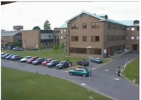
Described algorithms were tested using the private video bases and public domain video bases like PETS (PETS video database, n.d.), ETISEO (ETISEO video database, n.d.). Typical screen-shot of object tracking visualization is presented on Figure 4.
We created an algorithm analyzing and testing block that is based on comparison of automatic object detection and tracking results with results of manual object marking. Performance is measured
jects traced by the algorithm to all number of objects traced by algorithm. Simply put, 100% minus precision is a percentage of outliers provided by algorithm. The “Recall” equals is a percent-age ratio of human-marked objects found by the algorithm to all number of human-marked objects in a sequence, i.e. 100% minus recall means percentage of real objects that were not found by the algorithm somehow.
The table 1 contains some video sequences from PETS and ETISEO databases and corresponding processing results. FPS was espe-cially estimated for budget PC configuration: Intel Atom N270 1600 MHz processor and 1 Gb of RAM memory.
6 CONCLUSION
The problem of automatic video analysis for object detection and tracking is the most significant algorithmic topic in the digital video surveillance. The new motion analysis and object tracking technique is presented. Motion analysis algorithms are based on forming and processing of multiple-regression pseudospectrums. The object detection and tracking scheme contains: detection of moving pixel groups based on pseudospectrum analysis; forming of object hypotheses and interframe object tracking; spatiotem-poral filtration of object motion parameters. Results of testing on public domain PETS and ETISEO video test beds are outlined.
REFERENCES
Anandan, P., 1989. A computational framework and an algorithm for the measurement of visual motion. Int. J. Comp. Vision 2, pp. 283–310.
Barron, J., Fleet, D. and Beauchemin, S., 1994. Performance of optical flow techniques. Internat. Jour. of Computer Vision 12(1), pp. 43–77.
Box, G., Jenkins, G. M. and Reinsel, G., 1994. Time series anal-ysis: Forecasting and control (3rd edition).
ETISEO video database, n.d. http://www-sop.inria.fr/orion/ETISEO/.
Gabor, D., 1946. Theory of communication. Journal of the Insti-tute of Electrical Engineers 93, pp. 429–457.
Heeger, D. J., 1988. Optical flow using spatiotemporal filters. Int. J. Comp. Vision 1, pp. 279–302.
Horn, B. K. P. and Schunck, B. G., 1981. Determining optical flow. Artificial Intelligence 17, pp. 185–203.
Nagel, H., 1983. Displacement vectors derived from second-order intensity variations in image sequences. CGIP 9, pp. 85– 117.
PETS video database, n.d. http://www.cvg.rdg.ac.uk/slides/pets.html.
Video name Frame dimensions Detection Type Precision Recall FPS PETS-2001-SEQ1-CAM1 768x576 Moving objects 80% (8/10) 100% (8/8) 110 PETS-2001-SEQ1-CAM2 768x576 Moving objects 88% (8/9) 100% (8/8) 109 PETS-2006-S1-T1-C3 720x576 Moving objects 74% (26/35) 85% (24/28) 115 ETISEO-VS2-BE-19-C2 768x576 Moving objects 100% (4/4) 100% (4/4) 110 ETISEO-VS1-AP-5-C5 720x576 Moving objects 88% (8/9) 100% (6/6) 124 ETISEO-VS1-AP-5-C7 720x576 Moving objects 100% (9/9) 100% (7/7) 124 ETISEO-VS2-BC-17-C1 640x480 New/diss. objects 66% (2/3) 100% (2/2) 142 ETISEO-VS1-BC-12-C1 640x480 New/diss. objects 100% (1/1) 100% (1/1) 144
Table 1: Video analysis algorithms testing results