MATLAB®
MATLAB®
An Introduction
with Applications
Fifth Edition
Amos Gilat
Department of Mechanical and Aerospace Engineering The Ohio State University
Publisher: Executive Editor: Editorial Assistant: Cover Designer:
Associate Production Manager:
Cover Image: Amos Gilat.
DonFowley Dan Sayre Jessica Knecht Kenji Ngieng Joyce Poh
Founded in 1807, John Wiley & Sons, Inc. has been a valued source ofknowledge and understanding for more than 200 years, helping people around the world meet their needs and fulfill their aspirations. Our company is built on a foundation of principles that include responsibility to the communities we serve and where we live and work. In 2008, we launched a Corporate Citizenship Initiative, a global effort to address the environmental, social, economic, and ethical challenges we face in our business. Among the issues we are addressing are carbon impact, paper specifications and procurement, ethical conduct within our business and among our vendors, and community and charitable support. For more information, please visit our website: www.wiley.com/go/citizenship.
Copyright © 2015, 2011 John Wiley & Sons, Inc. All rights reserved. No part of this publication may be reproduced, stored in a retrieval system or transmitted in any form or by any means, electronic, mechanical, photocopying, recording, scanning or otherwise, except as permitted under Sections 107 or 108 of the 1976 United States Copyright Act, without either the prior written permission of the Publisher, or authorization through payment of the appropriate per-copy fee to the Copyright Clearance Center, Inc., 222 Rosewood Drive, Danvers, MA 01923, website www.copyright.com. Requests to the Publisher for permission should be addressed to the Permissions Department, John Wiley & Sons, Inc., 111 River Street, Hoboken, NJ 07030-5774, (201)748-6011, fax (201)748-6008, website http://www .wiley. com/go/permissions.
Evaluation copies are provided to qualified academics and professionals for review purposes only, for use in their courses during the next academic year. These copies are licensed and may not be sold or transferred to a third party. Upon completion of the review period, please return the evaluation copy to Wiley. Return instructions and a free of charge return mailing label are available at www.wiley.com/go/returnlabel. If you have chosen to adopt this textbook for use in your course, please accept this book as your complimentary desk copy. Outside of the United States, please contact your local sales representative.
ISBN 978-1-118-62986-4 (paper)
Preface
MATLAB® is a very popular language for technical computing used by stu dents, engineers, and scientists in universities, research institutes, and industries all over the world. The software is popular because it is powerful and easy to use. For university freshmen in it can be thought of as the next tool to use after the graphic calculator in high school.
This book was written following several years of teaching the software to freshmen in an introductory engineering course. The objective was to write a book that teaches the software in a friendly, non-intimidating fashion. Therefore, the book is written in simple and direct language. In many places bullets, rather than lengthy text, are used to list facts and details that are related to a specific topic. The book includes numerous sample problems in mathematics, science, and engi neering that are similar to problems encountered by new users ofMATLAB.
This fifth edition of the book is updated to MATLAB Release 2013b. In addition, the end of chapter problems have been revised. In Chapters 1 through 8 close to 80% of the problems are new or different than in previous editions.
I would like to thank several of my colleagues at The Ohio State University. Professor Richard Freuler for his comments, and Dr. Mike Parke for reviewing sections of the book and suggested modifications. I also appreciate the involve ment and support of Professors Robert Gustafson, John Demel and Dr. John Mer rill from the Engineering Education Innovation Center at The Ohio State University. Special thanks go to Professor Mike Lichtensteiger (OSU), and my daughter Tal Gilat (Marquette University), who carefully reviewed the first edi tion of the book and provided valuable comments and criticisms. Professor Brian Harper (OSU) has made a significant contribution to the new end of chapter prob lems in the present edition.
vi
I hope that the book will be useful and will help the users of MATLAB to enjoy the software.
Amos Gilat Columbus, Ohio November, 2013 gilat.l @osu.edu
To my parents Schoschana and Haim Gelbwacks
Contents
Preface v Introduction 1
Chapter 1 Starting with MATLAB 5
1.1 STARTING MATLAB, MATLAB WINDOWS 5 1.2 WORKING IN THE COMMAND WINDOW 9 1.3 ARITHMETIC OPERATIONS WITH SCALARS 11
1.3.1 Order of Precedence 11
1.3.2 Using MATLAB as a Calculator 12 1.4 DISPLAY FORMATS 12
1.5 ELEMENTARY MATH BUILT-IN FUNCTIONS 14 1.6 DEFINING SCALAR VARIABLES 16
1.6.1 The Assignment Operator 16 1.6.2 Rules About Variable Names 18 1.6.3 Predefined Variables and Keywords 19
1.7 USEFUL COMMANDS FOR MANAGING VARIABLES 19 1.8 SCRIPT FILES 20
1.8.1 Notes About Script Files 20
1.8.2 Creating and Saving a Script File 21 1.8.3 Running (Executing) a Script File 22 1.8.4 Current Folder 22
1.9 EXAMPLES OF MATLAB APPLICATIONS 24 1.10 PROBLEMS 27
Chapter 2 Creating Arrays 35
2.1 CREATING A ONE-DIMENSIONAL ARRAY (VECTOR) 35 2.2 CREATING A TwO-DIMENSIONAL ARRAY (MATRIX) 39
2.2.1 The zeros, ones and, eye Commands 40 2.3 NOTES ABOUT VARIABLES IN MATLAB 41 2.4 THE TRANSPOSE OPERATOR 41
2.5 ARRAY ADDRESSING 42 2.5.1 Vector 42
2.5.2 Matrix 43
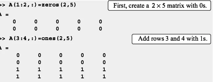
2.6 USING A COLON : IN ADDRESSING ARRAYS 44 2.7 ADDING ELEMENTS TO EXISTING VARIABLES 46 2.8 DELETING ELEMENTS 48
2.9 BUILT-IN FUNCTIONS FOR HANDLING ARRAYS 49 2.10 STRINGS AND STRINGS AS VARIABLES 53
2.11 PROBLEMS 55
Chapter 3 Mathematical Operations with Arrays 63 3.1 ADDITION AND SUBTRACTION 64
3.2 ARRAYMULTIPLICATION 65 3.3 ARRAY DIVISION 68
viii Contents
3.4 ELEMENT-BY-ELEMENT OPERATIONS 72
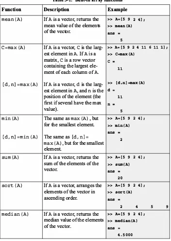
3.5 USING ARRAYS IN MATLAB BUILT-IN MATH FUNCTIONS 75 3.6 BUILT-IN FUNCTIONS FOR ANALYZING ARRAYS 75
3.7 GENERATION OF RANDOM NUMBERS 77 3.8 EXAMPLES OF MATLAB APPLICATIONS 80 3.9 PROBLEMS 86
Chapter 4 Using Script Files and Managing Data 95
4.1 THE MATLAB WORKSPACE AND THE WORKSPACE WINDOW 96 4.2 INPUT TO A SCRIPT FILE 97
4.3 OUTPUT COMMANDS 100 4.3.1 The disp Command 101 4.3.2 The fprintf Command 103 4.4 THE save AND load COMMANDS 111
4.4.1 The save Command 111 4.4.2 The load Command 112
4.5 IMPORTING AND EXPORTING DATA 114
4.5.1 Commands for Importing and Exporting Data 114 4.5.2 Using the Import Wizard 116
4.6 EXAMPLES OF MATLAB APPLICATIONS 118 4. 7 PROBLEMS 123
Chapter 5 Two-Dimensional Plots 133 5.1 THE plot COMMAND 134
5.1.1 Plot of Given Data 138 5.1.2 Plot of a Function 139 5.2 THE fplot COMMAND 140
5.3 PLOTTING MULTIPLE GRAPHS IN THE SAME PLOT 141 5.3.1 Using the plot Command 141
5.3.2 Using the hold on and hold off Commands 142 5.3.3 Using the line Command 143
5.4 FORMATTING A PLOT 144
5.4.1 Formatting a Plot Using Commands 144 5.4.2 Formatting a Plot Using the Plot Editor 148 5.5 PLOTS WITH LOGARITHMIC AxES 149
5.6 PLOTS WITH ERROR BARS 150 5.7 PLOTS WITH SPECIAL GRAPHICS 152 5.8 HISTOGRAMS 153
5.9 POLAR PLOTS 156
5.10 PuTTING MULTIPLE PLOTS ON THE SAME PAGE 157 5.11 MULTIPLE FIGURE WINDOWS 157
Contents ix
Chapter 6 Programming in MATLAB 175 6.1 RELATIONAL AND LOGICAL OPERATORS 176 6.2 CONDITIONAL STATEMENTS 184
6.2.1 The if-end Structure 184 6.2.2 The if-else-end Structure 186
6.2.3 The if-elseif-else-end Structure 187 6.3 THE switch-case STATEMENT 189
6.4 LOOPS 192
6.4.1 for-end Loops 192 6.4.2 while-end Loops 197
6.5 NESTED LOOPS AND NESTED CONDITIONAL STATEMENTS 200 6.6 THE break AND continue COMMANDS 202
6.7 EXAMPLES OF MATLAB APPLICATIONS 203 6.8 PROBLEMS 211
Chapter 7 User-Defined Functions and Function Files 221 7.1 CREATING A FUNCTION FILE 222
7.2 STRUCTURE OF A FUNCTION FILE 223 7.2.1 Function Definition Line 224 7.2.2 Input and Output Arguments 224 7.2.3 The H1 Line and Help Text Lines 226 7.2.4 Function Body 226
7.3 LOCAL AND GLOBAL VARIABLES 226 7.4 SAVING A FUNCTION FILE 227
7.5 USING A USER-DEFINED FUNCTION 228
7.6 EXAMPLES OF SIMPLE USER-DEFINED FUNCTIONS 229
7.7 COMPARISON BETWEEN SCRIPT FILES AND FUNCTION FILES 231 7.8 ANONYMOUS FUNCTIONS 231
7.9 FUNCTION FUNCTIONS 234
7.9 .1 Using Function Handles for Passing a Function into a Function Function 235
7.9.2 Using a Function Name for Passing a Function into a Function Function 238
7.10 SUBFUNCTIONS 240 7.11 NESTED FUNCTIONS 242
7.12 EXAMPLES OF MATLAB APPLICATIONS 245 7.13 PROBLEMS 248
Chapter 8 Polynomials, Curve Fitting, and Interpolation 261 8.1 POLYNOMIALS 261
8.1.1 Value of a Polynomial 262 8.1.2 Roots of a Polynomial 263
8.1.3 Addition, Multiplication, and Division of Polynomials 264 8.1.4 Derivatives ofPolynomials 266
8.2 CURVE FITTING 267
x Contents
8.3 INTERPOLATION 274
8.4 THE BASIC FITTING INTERFACE 278
8.5 EXAMPLES OF MATLAB APPLICATIONS 281 8.6 PROBLEMS 286
Chapter 9 Applications in Numerical Analysis 295 9.1 SOLVING AN EQUATION WITH ONE VARIABLE 295
9.2 FINDING A MINIMUM OR A MAXIMUM OF A FUNCTION 298 9.3 NUMERICAL INTEGRATION 300
9.4 ORDINARY DIFFERENTIAL EQUATIONS 303 9.5 EXAMPLES OF MATLAB APPLICATIONS 307 9.6 PROBLEMS 313
Chapter 10 Three-Dimensional Plots 323 10.1 LINE PLOTS 323
10.2 MESH AND SURFACE PLOTS 324 10.3 PLOTS WITH SPECIAL GRAPHICS 331 10.4 THE view COMMAND 333
10.5 EXAMPLES OF MATLAB APPLICATIONS 336 10.6 PROBLEMS 341
Chapter 11 Symbolic Math 347
11.1 SYMBOLIC OBJECTS AND SYMBOLIC EXPRESSIONS 348 11.1.1 Creating Symbolic Objects 348
11.1.2 Creating Symbolic Expressions 350
11.1.3 The fmdsym Command and the Default Symbolic Variable 353
11.2 CHANGING THE FORM OF AN EXISTING SYMBOLIC EXPRESSION 354 11.2.1 The collect, expand, and factor Commands 354 11.2.2 The simplify and simple Commands 356
11.2.3 The pretty Command 357 11.3 SOLVING ALGEBRAIC EQUATIONS 358 11.4 DIFFERENTIATION 363
11.5 INTEGRATION 365
11.6 SOLVING AN ORDINARY DIFFERENTIAL EQUATION 366 11.7 PLOTTING SYMBOLIC EXPRESSIONS 369
11.8 NUMERICAL CALCULATIONS WITH SYMBOLIC EXPRESSIONS 372 11.9 EXAMPLES OF MATLAB APPLICATIONS 376
11.10 PROBLEMS 384
Appendix: Summary of Characters, Commands, and Functions 393
Answers to Selected Problems www.wiley.com/college/gilat
Introduction
MATLAB is a powerful language for technical computing. The name MATLAB stands for MATrix LABoratory, because its basic data element is a matrix (array). MATLAB can be used for math computations, modeling and simulations, data analysis and processing, visualization and graphics, and algorithm development.
MATLAB is widely used in universities and colleges in introductory and advanced courses in mathematics, science, and especially engineering. In industry the software is used in research, development, and design. The standard MATLAB program has tools (functions) that can be used to solve common problems. In addition, MATLAB has optional toolboxes that are collections of specialized programs designed to solve specific types of problems. Examples include toolboxes for signal processing, symbolic calculations, and control systems.
Until recently, most of the users of MATLAB have been people with previous knowledge of programming languages such as FORTRAN and C who switched to MATLAB as the software became popular. Consequently, the majority of the literature that has been written about MATLAB assumes that the reader has knowledge of computer programming. Books about MATLAB often address advanced topics or applications that are specialized to a particular field. Today, however, MATLAB is being introduced to college students as the first (and often the only) computer program they will learn. For these students there is a need for a book that teaches MATLAB assuming no prior experience in computer programming.
The of This Book
MATLAB: An Introduction with Applications is intended for students who are using MATLAB for the first time and have little or no experience in computer programming. It can be used as a textbook in freshmen engineering courses or in workshops where MATLAB is being taught. The book can also serve as a reference in more advanced science and engineering courses where MATLAB is used as a tool for solving problems. It also can be used for self-study ofMATLAB by students and practicing engineers. In addition, the book can be a supplement or a secondary book in courses where MATLAB is used but the instructor does not have the time to cover it extensively.
Covered
MATLAB is a huge program, and therefore it is impossible to cover all of it in one book. This book focuses primarily on the foundations of MATLAB. The
2 Introduction
assumption is that once these foundations are well understood, the student will be able to learn advanced topics easily by using the information in the Help menu.
The order in which the topics are presented in this book was chosen carefully, based on several years of experience in teaching MATLAB in an introductory engineering course. The topics are presented in an order that allows the student to follow the book chapter after chapter. Every topic is presented completely in one place and then used in the following chapters.
The first chapter describes the basic structure and features of MATLAB and how to use the program for simple arithmetic operations with scalars as with a calculator. Script files are introduced at the end of the chapter. They allow the student to write, save, and execute simple MATLAB programs. The next two chapters are devoted to the topic of arrays. MATLAB's basic data element is an array that does not require dimensioning. This concept, which makes MATLAB a very powerful program, can be a little difficult to grasp for students who have only limited knowledge of and experience with linear algebra and vector analysis. The concept of arrays is introduced gradually and then explained in extensive detail. Chapter 2 describes how to create arrays, and Chapter 3 covers mathematical operations with arrays.
Following the basics, more advanced topics that are related to script files and input and output of data are presented in Chapter 4. This is followed by coverage of two-dimensional plotting in Chapter 5. Programming with MATLAB is introduced in Chapter 6. This includes flow control with conditional statements and loops. User-defmed functions, anonymous functions, and function functions are covered next in Chapter 7. The coverage of function files (user-defmed functions) is intentionally separated from the subject of script files. This has proven to be easier to understand by students who are not familiar with similar concepts from other computer programs.
The next three chapters cover more advanced topics. Chapter 8 describes how MATLAB can be used for carrying out calculations with polynomials, and how to use MATLAB for curve fitting and interpolation. Chapter 9 covers applications of MATLAB in numerical analysis. It includes solving nonlinear equations, finding minimum or a maximum of a function, numerical integration, and solution of first-order ordinary differential equations. Chapter 10 describes how to produce three-dimensional plots, an extension of the chapter on two dimensional plots. Chapter 11 covers in great detail how to use MATLAB in symbolic operations.
The Framework of a
Introduction
tutorials in order to gain experience in using MATLAB. In addition, every chapter includes formal sample problems that are examples of applications of MATLAB for solving problems in math, science, and engineering. Each example includes a problem statement and a detailed solution. Some sample problems are presented in the middle of the chapter. All of the chapters (except Chapter 2) have a section at the end with several sample problems of applications. It should be pointed out that problems with MATLAB can be solved in many different ways. The solutions of the sample problems are written such that they are easy to follow. This means that in many cases the problem can be solved by writing a shorter, or sometimes "trickier," program. The students are encouraged to try to write their own solu tions and compare the end results. At the end of each chapter there is a set of homework problems. They include general problems from math and science and problems from different disciplines of engineering.
Calculations
MATLAB is essentially a software for numerical calculations. Symbolic math operations, however, can be executed if the Symbolic Math toolbox is installed. The Symbolic Math toolbox is included in the student version of the software and can be added to the standard program.
Software and Hardware
The MATLAB program, like most other software, is continually being developed and new versions are released frequently. This book covers MATLAB Version 8.2.0.701, Release 2013b. It should be emphasized, however, that the book covers the basics of MATLAB, which do not change much from version to version. The book covers the use of MATLAB on computers that use the Windows operating system. Everything is essentially the same when MATLAB is used on other machines. The user is referred to the documentation of MATLAB for details on using MATLAB on other operating systems. It is assumed that the software is installed on the computer, and the user has basic knowledge of operating the computer.
The Order of in the Book
It is probably impossible to write a textbook where all the subjects are presented in an order that is suitable for everyone. The order of topics in this book is such that the fundamentals ofMATLAB are covered first (arrays and array operations), and, as mentioned before, every topic is covered completely in one location, which makes the book easy to use as a reference. The order of the topics in this fifth edition is the same as in the previous edition. Programming is introduced before user-defmed functions. This allows using programming in user-defmed functions. Also, applications ofMATLAB in numerical analysis follow Chapter 8 which covers polynomials, curve fitting, and interpolation.
Chapterl
Starting with
MATLAB
This chapter begins by describing the characteristics and purpose of the different windows in MATLAB. Next, the Command Window is introduced in detail. The chapter shows how to use MATLAB for arithmetic operations with scalars in much to the way that a calculator is used. This includes the use of elementary math functions with scalars. The chapter then shows how to define scalar vari ables (the assigmnent operator) and how to use these variables in arithmetic calcu lations. The last section in the chapter introduces script files. It shows how to write, save, and execute simple MATLAB programs.
1.1 STARTING MATLAB, MATLAB WINDOWS
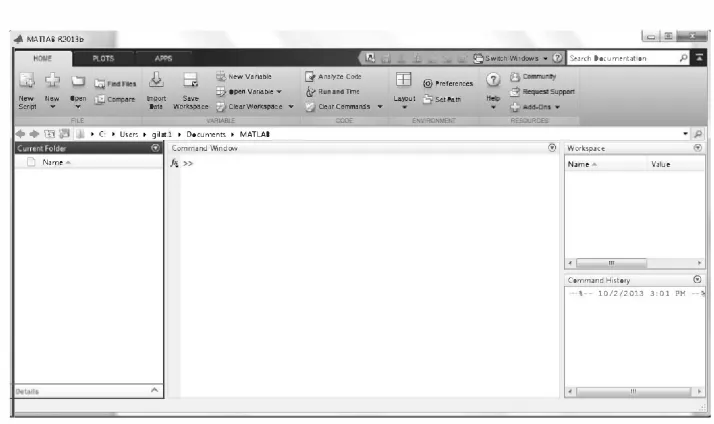
It is assumed that the software is installed on the computer, and that the user can start the program. Once the program starts, the MATLAB desktop window opens with the default layout, Figure 1-1. The layout has a Toolstrip at the top, the Cur rent Folder Toolbar below it, and four windows underneath. At the top of the
Toolstrip there are three tabs: HOME, PLOTS, and APPS. Clicking on the tabs changes the icons in the Toolstrip. Commonly, MATLAB is used with the HOME tab selected. The associated icons are used for executing various commands, as explained later in this chapter. The PLOTS tab can be used to create plots, as explained in Chapter 5 (Section 5.12), and the APPS tab can be used for opening additional applications and Toolboxes of MATLAB.
The default layout
The default layout (Figure 1-1) consists of the following four windows that are displayed under the Toolstrip: the Command Window (larger window at the cen ter), the Current Folder Window (on the left) and the Workspace and Command History windows (on the right). A list of several MATLAB windows and their purposes is given in Table 1-1.
Four of the windows-the Command Window, the Figure Window, the Editor Window, and the Help Window-are used extensively throughout the book and
6
, ..;. MATl.AB R20Bb
r«rw New Open Script • ..,.
db a;, <ow"'"'" Open Vlll'l!ltlole ,.. hiport s.r.ve
011111 W!llb{wlce ClearWortspllr:e '9' • + [J'] � C: � U�m � gilat1 • Document� • MATLAB.
(ommandWindow
D
Name-1: with MATLAB
Clsw:tdlWI'll»ws .. Starch Documentation (]> An11lyze cooe III
£ir.RunandTrne @Preferences " Cle.!lrCo!Tinllnds ,... Laywt �tPath
® Worlupace Name .a. Value
CommandHistory @ · ·ls--10/2/2013 3:01 PM
--Figure 1-1: The default view ofMATLAB desktop.
are briefly described on the following pages. More detailed descriptions are included in the chapters where they are used. The Command History Window, Current Folder Window, and the Workspace Window are described in Sections 1.2, 1.8.4, and 4.1, respectively.
Command Window: The Command Window is MATLAB 's main window and opens when MATLAB is started. It is convenient to have the Command Window as the only visible window. This can be done either by closing all the other win dows, or by selecting Command Window Only in the menu that opens when the Layout icon on the Toolstrip is selected. To close a window, click on the pull down menu at the top right-hand side of the window and then select Close. Work ing in the Command Window is described in detail in Section 1.2.
Table 1-1: MATLAB windows
Window Purpose
Command Window Main window, enters variables, runs programs.
Figure Window Contains output from graphic commands.
Editor Window Creates and debugs script and function files.
Help Window Provides help information.
1.1 MATLAB Windows
Table 1-1: MATLAB windows
Window Purpose
Workspace Window Provides information about the variables that are stored.
Current Folder Window Shows the files in the current folder.
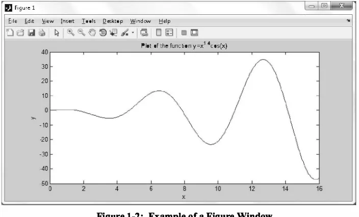
Figure Window: The Figure Window opens automatically when graphics com mands are executed, and contains graphs created by these commands. An example of a Figure Window is shown in Figure 1-2. A more detailed description of this window is given in Chapter 5.
IJ Figur� 1
file ,Edit Yiew Insert Iools. Q.esktop Window Help
Plot of the function y� 1 4cos(x)
30 20 10
-10 - 20 -30 -40
Figure 1-2: Example of a Figure Window.
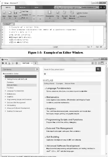
Editor Window: The Editor Window is used for writing and editing programs. This window is opened by clicking on the New Script icon in the Toolstrip, or by clicking on the New icon and then selecting Script from the menu that opens. An example of an Editor Window is shown in Figure 1-3. More details on the Editor Window are given in Section 1.8.2, where it is used for writing script files, and in Chapter 7, where it is used to write function files.
Help Window: The Help Window contains help information. This window can be opened from the Help icon in the Toolstrip of the Command Window or the toolbar of any MATLAB window. The Help Window is interactive and can be used to obtain information on any feature ofMATLAB. Figure 1-4 shows an open Help Window.
When MATLAB is started for the first time, the screen looks like that shown in Figure 1-1. For most beginners it is probably more convenient to close all the
8 > Getting Started wilh MA Tl.AB
Examples
> Programming Scripls and Functions > Data and File Management > GUI Building
> Advanced Software Development > De5ktop Environmenl
Search Documentation
MATLAB
GeHing Started Examples Release No1es > Language Fundamentals
SyrJta,;, opera!OJs, data types, array irKfexing aOO m.:mipul.alioo
> Mathematics
UneM algebra. basic statistics, differentiation aOO integrals, Fourier tr.:msforrns, -arKI other mathematics
> Graphics
Two- alllf three-dimensiooal plol.s, dala exploration and visualiz.alion techniques, images, printing, arK! graphics objects
> Programming Scripts and Functions Program Iiies, control now, edltir�g, debugging
> Data and File Management Data import and exp<Ht, wort.space, li!€5 and folders
> GUI Building
Application development usillQ GUIDE alld callbac:ks
> Advanced Software Development
Objecl-orienled programming; code performance; unit testing; mterfaces to
Java"', CIC+t-, .NET and other la�uage:s file:/1/C:/Proqram F11es/MATLAB/R2013b/help/matlab/relea<e-note<.html
1.2 in the Command Window
windows except the Command Window. The closed windows can be reopened by selecting them from the layout icon in the Toolstrip. The windows shown in Fig ure 1-1 can be displayed by clicking on the layout icon and selecting Default in the menu that opens. The various windows in Figure 1-1 are docked to the desk top. A window can be undocked (become a separate, independent window) by dragging it out. An independent window can be redocked by clicking on the pull down menu at the top right-hand side of the window and then selecting Dock.
1.2 WORKING IN THE COMMAND WINDOW
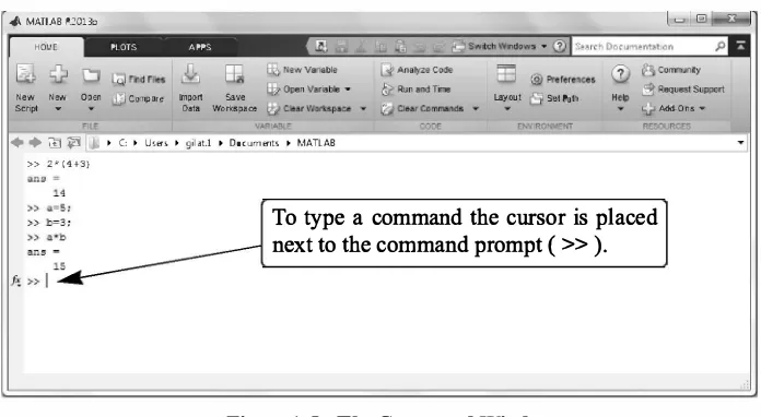
The Command Window is MATLAB's main window and can be used for execut ing commands, opening other windows, running programs written by the user, and managing the software. An example of the Command Window, with several sim ple commands that will be explained later in this chapter, is shown in Figure 1-5 .
..JJ. MA.TlAB R2013b
HOME PLOTS APPS
New New Open ]= CofTllare rnport Save
Scr'p: .. om WorKspace Layout Se!Path + • rn � � C: � Users � gil.rtl ,. Doc:uments � MATLAB
>> 2"" (1+3}
To type a command the cursor is placed next to the command prompt ( >> ).
Figure 1-5: The Command Window.
Notes for working in the Command Window:
Add-OM •
• To type a command, the cursor must be placed next to the command prompt ( >> ). • Once a command is typed and the Enter key is pressed, the command is executed.
However, only the last command is executed. Everything executed previously (that might be still displayed) is unchanged.
• Several commands can be typed in the same line. This is done by typing a comma
between the commands. When the Enter key is pressed, the commands are exe cuted in order from left to right.
• It is not possible to go back to a previous line that is displayed in the Command
Window, make a correction, and then re-execute the command.
10 1: with MATLAB
• A previously typed command can be recalled to the command prompt with the up arrow key ( t ). When the command is displayed at the command prompt, it can be modified if needed and then executed. The down-arrow key ( .t) can be used to move down the list of previously typed commands.
• If a command is too long to fit in one line, it can be continued to the next line by typing three periods ... (called an ellipsis) and pressing the Enter key. The con tinuation of the command is then typed in the new line. The command can con tinue line after line up to a total of 4,096 characters.
The semicolon ( ; ):
When a command is typed in the Command Window and the Enter key is pressed, the command is executed. Any output that the command generates is dis played in the Command Window. If a semicolon ( ; ) is typed at the end of a com mand, the output of the command is not displayed. Typing a semicolon is useful when the result is obvious or known, or when the output is very large.
If several commands are typed in the same line, the output from any of the commands will not be displayed if a semicolon instead of a comma is typed between the commands.
Typing%:
When the symbol% (percent) is typed at the beginning of a line, the line is desig nated as a comment. This means that when the Enter key is pressed the line is not executed. The% character followed by text (comment) can also be typed after a command (in the same line). This has no effect on the execution of the command. Usually there is no need for comments in the Command Window. Comments, however, are frequently used in a program to add descriptions or to explain the program (see Chapters 4 and 6).
The c l c command:
The clc command (type clc and press Enter) clears the Command Window. After typing in the Command Window for a while, the display may become very long. Once the clc command is executed, a clear window is displayed. The com mand does not change anything that was done before. For example, if some vari ables were defined previously (see Section 1.6), they still exist and can be used. The up-arrow key can also be used to recall commands that were typed before. The Command History Window:
1.3 Arithmetic with Scalars
then right-clicking the mouse and selecting Delete Selection. The whole history can be deleted by right-clicking the mouse and selecting choose Clear Command History in the menu that opens.
1.3 ARITHMETIC OPERATIONS WITH SCALARS
In this chapter we discuss only arithmetic operations with scalars, which are num bers. As will be explained later in the chapter, numbers can be used in arithmetic calculations directly (as with a calculator) or they can be assigned to variables, which can subsequently be used in calculations. The symbols of arithmetic opera tions are:
Addition + 5+3
Subtraction 5-3
Multiplication * 5*3
Right division I 5/3
Left division \ 5\3=3/5
Exponentiation A 5 A 3 (means 53= 125)
It should be pointed out here that all the symbols except the left division are the same as in most calculators. For scalars, the left division is the inverse of the right division. The left division, however, is mostly used for operations with arrays, which are discussed in Chapter 3.
1.3.1 Order of Precedence
MATLAB executes the calculations according to the order of precedence dis played below. This order is the same as used in most calculators.
Precedence First
Second
Third
Fourth
Mathematical
Parentheses. For nested parentheses, the innermost are executed ftrst.
Exponentiation.
Multiplication, division (equal precedence).
Addition and subtraction.
In an expression that has several operations, higher-precedence operations are executed before lower-precedence operations. If two or more operations have the same precedence, the expression is executed from left to right. As illustrated in the next section, parentheses can be used to change the order of calculations.
12 1: with MATLAB
1.3.2 Using MATLAB as a Calculator
The simplest way to use MATLAB is as a calculator. This is done in the Com mand Window by typing a mathematical expression and pressing the Enter key. MATLAB calculates the expression and responds by displaying ans = followed by the numerical result of the expression in the next line. This is demonstrated in Tutorial 1-1.
Tutorial1-1: Using MATLAB as a calculator .
» 7+8/2
5A3 is executed first, /2 is executed next.
1/3 is executed frrst, 27A(1/3) and 32A0.2 are
continue the expression on the next line.
The last expression is the first four terms of the Taylor series for sin(1t/4).
1.4 Formats
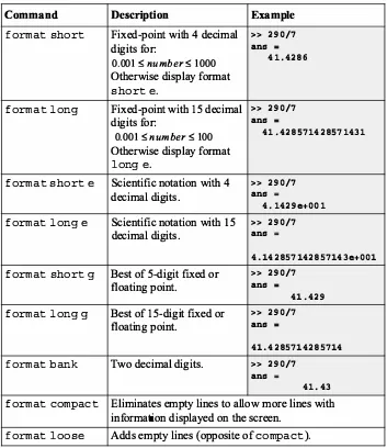
changed with the format command. Once the format command is entered, all the output that follows is displayed in the specified format. Several of the avail able formats are listed and described in Table 1-2.
MATLAB has several other formats for displaying numbers. Details of these formats can be obtained by typing help format in the Command Window. The format in which numbers are displayed does not affect how MATLAB computes and saves numbers.
Table 1-2: Display formats
Command Description Example
format short Fixed-point with 4 decimal » 290/7
digits for: ans =
0.001 :5: number :5: 1000 41.4286 Otherwise display format
short e.
format long Fixed-point with 15 decimal » 290/7
digits for: ans =
0.001 :5: number :5: 100 41.428571428571431 Otherwise display format
long e.
format short e Scientific notation with 4 » 290/7
decimal digits. ans =
4.1429e+001 format long e Scientific notation with 15 » 290/7
decimal digits. ans =
4.142857142857143e+001 format short g Best of 5-digit fixed or » 290/7
floating point. ans =
41.429 format long g Best of 15-digit fixed or » 290/7
floating point. ans =
41.4285714285714 format bank Two decimal digits. » 290/7
ans =
41.43 format compact Eliminates empty lines to allow more lines with
information displayed on the screen.
format loose Adds empty lines (opposite of compact).
14 1: with MATLAB
1.5 ELEMENTARY MATH BUILT-IN FUNCTIONS
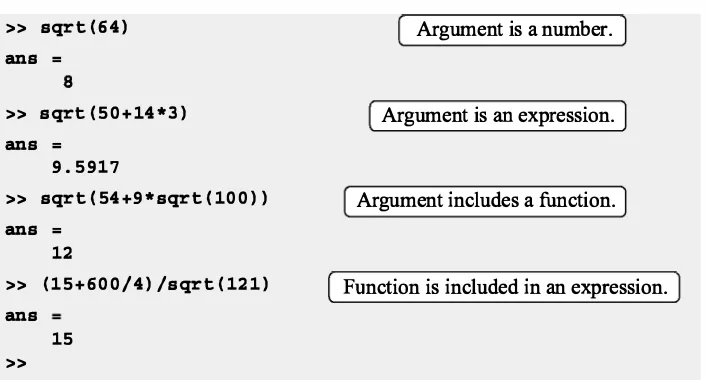
In addition to basic arithmetic operations, expressions in MATLAB can include functions. MATLAB has a very large library of built-in functions. A function has a name and an argument in parentheses. For example, the function that calculates the square root of a number is sqrt (x). Its name is sqrt, and the argument is x. When the function is used, the argument can be a number, a variable that has been assigned a numerical value (explained in Section 1.6), or a computable expression that can be made up of numbers and/or variables. Functions can also be included in arguments, as well as in expressions. Tutorial1-2 shows examples of using the function sqrt (x) when MATLAB is used as a calculator with sca lars.
Tutorial1-2: Using the sqrt built-in function.
>> sqrt(64) ans =
>> sqrt(50+14*3) ans =
9.5917
Argument is a number.
Argument is an expression.
>> sqrt(54+9*sqrt(100)) Argument includes a function. ans =
12
>> (15+600/4)/sqrt(121) Function is included in an expression. ans
15 >>
Some commonly used elementary MATLAB mathematical built-in functions are given in Tables 1-3 through 1-5. A complete list of functions organized by cat egory can be found in the Help Window.
Table 1-3: Elementary math functions
Function Description Example
sqrt(x) Square root. » sqrt (81)
ans =
nthroot(x,n) Real nth root of a real number x. >> nthroot(80,5) (If x is negative n must be an ans =
odd integer.) 2.4022
exp(x) Exponential (eX) . >> exp (5) ans =
1.5 Math Built-in Functions
Table 1-3: Elementary math functions (Continued)
Function Description Example
abs (x) Absolute value. >> abs(-24)
ans = 24
log(x) Natural logarithm. » log (1000)
Base e logarithm (In). ans = 6.9078
loglO (x) Base 10 logarithm. » log10 (1000)
ans = 3.0000 factorial(x) The factorial function x! >> factorial(5)
(x must be a positive integer.) ans = 120 Table 1-4: Trigonometric math functions
Function Description Example
sin(x) Sine of angle x (x in radians). » sin (pi/6) sind(x) Sine of angle x (x in degrees). ans =
0.5000 cos (x) Cosine of angle x (x in radians). >> cosd(30) cosd(x) Cosine of angle x (x in degrees). ans =
0.8660 tan(x) Tangent of angle x (x in radians). » tan (pi/6) tand(x) Tangent of angle x (x in degrees). ans =
0.5774 cot(x) Cotangent of angle x (x in radians). » cotd(30) cotd(x) Cotangent of angle x (x in degrees). ans =
1. 7321
The inverse trigonometric functions are asin (x), acos (x), a tan (x), acot (x) for the angle in radians; and asind (x), acosd (x), atand (x), acotd (x) for the angle in degrees. The hyperbolic trigonometric functions are sinh (x), cosh (x), tanh (x), and coth (x) . Table 1-4 uses pi, which is equal to 1t (see Section 1.6.3).
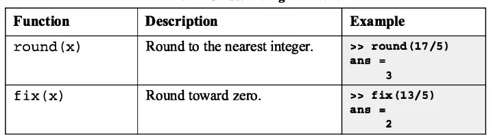
Table 1-5: Rounding functions
Function Description Example
round(x) Round to the nearest integer. » round (17 /5) ans =
3
fix(x) Round toward zero. » fix(13/5)
ans = 2
16 1: with MATLAB
Table 1-5: Rounding functions (Continued)
Function Description Example
ceil (x) Round toward infinity. » ceil (11/5)
ans = 3
floor(x) Round toward minus infinity. » floor (-9/4) ans =
-3 rem(x,y) Returns the remainder after x is >> rem(13,5)
divided by y. ans =
3 sign(x) Signum function. Returns 1 if » sign (5)
x>0 ,-1 ifx<O,andOif ans =
X = 0. 1
1.6 DEFINING SCALAR VARIABLES
A variable is a name made of a letter or a combination of several letters (and dig its) that is assigned a numerical value. Once a variable is assigned a numerical value, it can be used in mathematical expressions, in functions, and in any MAT LAB statements and commands. A variable is actually a name of a memory loca tion. When a new variable is defined, MATLAB allocates an appropriate memory space where the variable's assignment is stored. When the variable is used the stored data is used. If the variable is assigned a new value the content of the memory location is replaced. (In Chapter 1 we consider only variables that are assigned numerical values that are scalars. Assigning and addressing variables that are arrays is discussed in Chapter 2.)
1.6.1 The Assignment Operator
In MATLAB the = sign is called the assignment operator. The assignment opera tor assigns a value to a variable.
Variable_ name = A numerical value, or a computable expression
• The left-hand side of the assignment operator can include only one variable name. The right-hand side can be a number, or a computable expression that can include numbers and/or variables that were previously assigned numerical values. When the Enter key is pressed the numerical value of the right-hand side is assigned to the variable, and MATLAB displays the variable and its assigned value in the next two lines.
1.6 Scalar Variables MATLAB displays the variable name and its assigned value.
A new value is assigned to x. The
Assign the value of the expres sion on the right-hand side to the variable C.
• If a semicolon is typed at the end of the command, then when the Enter key is pressed, MATLAB does not display the variable with its assigned value (the vari able still exists and is stored in memory).
• If a variable already exists, typing the variable's name and pressing the Enter key will display the variable and its value in the next two lines.
As an example, the last demonstration is repeated below using semicolons.
>> a=12; >> B=4;
>> C=(a-B)+40-a/B*10;
The variables a, B, and C are defined but are not displayed, since a semicolon is typed at the end of each statement.
>> c c =
18
The value of the variable C is displayed by typing the name of the variable.
• Several assignments can be typed in the same line. The assignments must be sepa rated with a comma (spaces can be added after the comma). When the Enter key is pressed, the assignments are executed from left to right and the variables and
18 1: with MATLAB
their assignments are displayed. A variable is not displayed if a semicolon is typed instead of a comma. For example, the assignments of the variables a, B, and C above can all be done in the same line.
>> a=12, B=4; C=(a-B)+40-a/B*10
a 12
18
The variable B is not displayed because a semi colon is typed at the end of the assignment.
• A variable that already exists can be reassigned a new value. For example: >> ABB=72; value of72 is assigned to the variable ABE. >> ABB=9; A new value of9 is assigned to the variable ABE. >>
ABB
>> ABB
9
The current value of the variable is dis played when the name of the variable is typed and the Enter key is pressed.
• Once a variable is defined it can be used as an argument in functions. For exam ple:
>> X=0.75;
>> E=sin(x)A2+cos(x)A2 E =
1
>>
1.6.2 Rules About Variable Names
A variable can be named according to the following rules: • Must begin with a letter.
• Can be up to 63 characters long.
• Can contain letters, digits, and the underscore character.
• Cannot contain punctuation characters (e.g., period, comma, semicolon).
• MATLAB is case-sensitive: it distinguishes between uppercase and lowercase let ters. For example, AA, Aa, aA, and aa are the names of four different variables. • No spaces are allowed between characters (use the underscore where a space is
desired).
1.7 Useful Commands for Variables
1.6.3 Predefined Variables and Keywords
There are 20 words, called keywords, that are reserved by MATLAB for various purposes and cannot be used as variable names. These words are:
break case
end for
persistent
catch classdef continue else
function global if otherwise
return spmd switch try while
elseif par for
When typed, these words appear in blue. An error message is displayed if the user tries to use a keyword as a variable name. (The keywords can be displayed by typ ing the command iskeyword.)
A number of frequently used variables are already defmed when MATLAB is started. Some of the predefmed variables are:
ans A variable that has the value of the last expression that was not assigned to a specific variable (see Tutoriall-1). If the user does not assign the value of an expression to a variable, MATLAB automatically stores the result in ans.
pi The number 1t.
eps The smallest difference between two numbers. Equal to 2A(-52), which is approximately 2.2204e-O 16.
inf Used for infmity.
i Defmed as ./-1, which is: 0 + l .OOOOi. j Same as i.
NaN Stands for Not-a-Number. Used when MATLAB cannot determine a valid numeric value. Example: 0/0.
The predefmed variables can be redefined to have any other value. The vari abies pi, eps, and inf, are usually not redefmed since they are frequently used in many applications. Other predefmed variables, such as i and j , are sometime redefined (commonly in association with loops) when complex numbers are not involved in the application.
1. 7 USEFUL COMMANDS FOR MANAGING VARIABLES
The following are commands that can be used to eliminate variables or to obtain information about variables that have been created. When these commands are typed in the Command Window and the Enter key is pressed, either they provide information, or they perform a task as specified below.
Command Outcome
clear Removes all variables from the memory.
20
Command
clear x y z
who
whos
1.8 SCRIPT FILES
Outcome
1: with MATLAB
Removes only variables x, y, and z from the memory.
Displays a list of the variables currently in the memory.
Displays a list of the variables currently in the memory and their sizes together with informa tion about their bytes and class (see Section 4.1 ).
So far all the commands were typed in the Command Window and were executed when the Enter key was pressed. Although every MATLAB command can be executed in this way, using the Command Window to execute a series of com mands-especially if they are related to each other (a program)-is not conve nient and may be difficult or even impossible. The commands in the Command Window cannot be saved and executed again. In addition, the Command Window is not interactive. This means that every time the Enter key is pressed only the last command is executed, and everything executed before is unchanged. If a change or a correction is needed in a command that was previously executed and the result of this command is used in commands that follow, all the commands have to be entered and executed again.
A different (better) way of executing commands with MA TLAB is first to create a file with a list of commands (program), save it, and then run (execute) the file. When the file runs, the commands it contains are executed in the order that they are listed. If needed, the commands in the file can be corrected or changed and the file can be saved and run again. Files that are used for this purpose are called script files.
IMPORTANT NOTE: This section covers only the minimum required in order to run simple programs. This will allow the student to use script mes when practicing the material that is presented in this and the next two chap ters (instead of typing repeatedly in the Command Window). Script mes are considered again in Chapter 4, where many additional topics that are essen tial for understanding MATLAB and writing programs in script me are cov ered.
1.8.1 Notes About Script Files
• A script file is a sequence ofMATLAB commands, also called a program.
1.8 Files
• When a script file has a command that generates an output (e.g., assignment of a value to a variable without a semicolon at the end), the output is displayed in the Command Window.
• Using a script file is convenient because it can be edited (corrected or other wise changed) and executed many times.
• Script files can be typed and edited in any text editor and then pasted into the MATLAB editor.
• Script files are also called M-files because the extension .m is used when they are saved.
1.8.2 Creating and Saving a Script File
In MA TLAB script files are created and edited in the Editor/Debugger Window. This window is opened from the Command Window by clicking on the New Script icon in the Toolstrip, or by clicking New in the Toolstrip and then selecting Script from the menu that open. An open Editor/Debugger Window is shown in Figure 1-6.
� Editor -Untitled
EDrTOR PUBLISH VIEW
Line number
NAVIGATE Breakpoints Run BREAKPOINTS
The commands in the script file are typed line by line. The lines are num bered automatically. A new line starts when the Enter key is pressed.
Figure 1-6: The Editor/Debugger Window.
The Editor/Debugger Window has a Toolstrip at the top and three tabs EDI TOR, PUBLISH, and VIEW above it. Clicking on the tabs changes the icons in the Toolstrip. Commonly, MATLAB is used with the HOME tab selected. The associated icons are used for executing various commands, as explained later in the Chapter. Once the window is open, the commands of the script file are typed line by line. MA TLAB automatically numbers a new line every time the Enter key is pressed. The commands can also be typed in any text editor or word proces sor program and then copied and pasted in the Editor/Debugger Window. An example of a short program typed in the Editor/Debugger Window is shown in Figure 1-7. The first few lines in a script file are typically comments (which are
22 1: with MATLAB
not executed, since the first character in the line is %) that describe the program written in the script file.
Editor-C:\MATLAB BQ()k 5th Edition\Chapter 1\Chapl_Examp_l.m
EDITOR PUBUSH VIEW
[{)J Find files Insert ®\ fx t'£J • Q
s 6 7 8
-�Go To • F1nd •
Figure 1-7: A program typed in the Editor/Debugger Window.
Before a script file can be executed it has to be saved. This is done by click ing Save in the Toolstrip and selecting Save As ... from the menu that opens. When saved, MA TLAB adds the extension .m to the name. The rules for naming a script file follow the rules of naming a variable (must begin with a letter, can include digits and underscore, no spaces, and up to 63 characters long). The names of user-defmed variables, predefined variables, and MATLAB commands or func tions should not be used as names of script files.
1.8.3 Running (Executing) a Script File
A script file can be executed either directly from the Editor Window by clicking on the Run icon (see Figure 1-7) or by typing the file name in the Command Win dow and then pressing the Enter key. For a file to be executed, MATLAB needs to know where the file is saved. The file will be executed if the folder where the file is saved is the current folder ofMATLAB or if the folder is listed in the search path, as explained next.
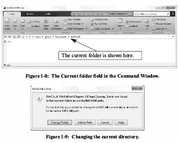
1.8.4 Current Folder
1.8 Files
.fA MATLAB R20Hb
HOME PLOTS APPS s��rch Docum�nt�tion
New New Open
The current folder is shown here.
Request Support He�
0Add-Ons •
Figure 1-8: The Current folder field in the Command Window.
MATlAB Edi1or
FileC:\...k 5th Editioo\Chapter 1\Chapl_Examp_l.m is oot louod in the current fokJer or on the MA TLAB path..
To run this. file,. you can either change the MATLAB current folder or add its. folder to the MATLAB path.
Figure 1-9: Changing the current directory.
Current Folder field in the Command Window. The current folder can also be changed in the Current Folder Window, shown in Figure 1-10, which can be opened from the Desktop menu. The Current Folder can be changed by choosing the drive and folder where the file is saved.
'+ MATIAB R2013o
Figure 1-10: The Current Folder Window.
Click here to change the folder.
24 1: with MATLAB
An alternative simple way to change the current folder is to use the cd com mand in the Command Window. To change the current folder to a different drive, type cd, space, and then the name of the directory followed by a colon: and press the Enter key. For example, to change the current folder to drive E (e.g., the flash drive) type cd E:. If the script file is saved in a folder within a drive, the path to that folder has to be specified. This is done by typing the path as a string in the cd command. For example, cd ( 1 E: \Chapter 1 1 ) sets the path to the folder Chapter 1 in drive F. The following example shows how the current folder is changed to be drive E. Then the script file from Figure 1-7, which was saved in drive E as ProgramExample.m, is executed by typing the name of the file and pressing the Enter key.
>> cd { 'E: \Chapter The current directory is changed to drive
>> Chapl_Exampl xl
3.5000 x2
-1.2500
The script file is executed by typing the name of the file and pressing the Enter key.
The output generated by the script file (the roots xl and x2) is displayed in the Command Window.
1.9 EXAMPLES OF MATLAB APPLICATIONS
Sample Problem 1-1: Trigonometric identity A trigonometric identity is given by:
cosz:! = tanx + sinx
2 2tanx
Verify that the identity is correct by calculating each side of the equation, substi-• 1t
tutmg x = 5.
Solution
The problem is solved by typing the following commands in the Command Win dow.
>> X=pi/5;
>> LHS=cos(x/2)A2 LHS =
0.9045
>> RHS=(tan(x)+sin(x))/(2*tan(x)) RHS
0.9045
Define x. Calculate the left-hand side.
1.9 of MATLAB
Sample Problem 1-2: Geometry and trigonometry
Four circles are placed as shown in the figure. At each point where two circles are in contact, they are tangent to each other. Determine the distance between the centers C2 and C4.
The radii of the circles are:
R1 = 16mm, R2 = 6.5mm, R3 = 12mm, and R4 = 9.5mm.
Solution
The lines that connect the centers of the circles create four triangles. In two of the triangles, AC1 C2C3 and AC1 C3C4, the lengths of all the sides are known. This information is used to calculate the angles y1 and y2 in these triangles by using the law of cosines. For example, y1 is calculated from:
(C2C3)2 = (C1C2)2+(C1C3)2-2(C1C2)(C1C3)cosy1 Next, the length of the side C2C4 is calculated by
considering the triangle AC1 C2C4. This is done, again, by using the law of cosines (the lengths cl Cz and cl c4 are known and the angle '¥3 is the sum of the angles 'YI and y2).
The problem is solved by writing the following program in a script file:
% Solution of Sample Problem 1-2
Rl=l6; R2=6.5; R3=12; R4=9.5;
ClC2=Rl+R2; ClC3=Rl+R3; ClC4=Rl+R4;
the R's. Calculate the lengths of the sides. C2C3=R2+R3; C3C4=R3+R4;
Gamal=acos((ClC2A2+ClC3A2-C2C3A2)/(2*ClC2*ClC3));
Gama2=acos((ClC3A2+ClC4A2-C3C4A2)/(2*ClC3*ClC4));
Gama3 =Gamal +Gama2 ;
C2C4=sqrt(ClC2A2+ClC4A2-2*ClC2*ClC4*cos(Gama3))
Calculate the length of side C2C4.
When the script file is executed, the following (the value of the variable C2C4) is displayed in the Command Window:
C2C4 = 33.5051
26
Sample Problem 1-3: Heat transfer
1: with MATLAB
An object with an initial temperature of T0 that is placed at time t = 0 inside a chamber that has a constant temperature of T3 will experience a temperature change according to the equation
T = T3+(T0-T3)e -kt
where Tis the temperature of the object at timet, and k is a constant. A soda can at a temperature of 120° F (after being left in the car) is placed inside a refrigerator where the temperature is 38°F. Determine, to the nearest degree, the temperature of the can after three hours. Assume k = 0.45. First define all of the variables and then calculate the temperature using one MATLAB command.
Solution
The problem is solved by typing the following commands in the Command Win dow.
>> Ts=38; T0=120; k=0.45; t=3;
>> T=round(Ts+(TO-Ts)*exp(-k*t))
T =
59 Round to the nearest integer.
Sample Problem 1-4: Compounded interest
The balance B of a savings account after t years when a principal P is invested at an annual interest rate r and the interest is compounded n times a year is given by:
B=P
(
t+�
r
t (1)If the interest is compounded yearly, the balance is given by:
B
=
P(l +r)t (2)Suppose $5,000 is invested for 17 years in one account for which the interest is compounded yearly. In addition, $5,000 is invested in a second account in which the interest is compounded monthly. In both accounts the interest rate is 8.5%. Use MATLAB to determine how long (in years and months) it would take for the balance in the second account to be the same as the balance of the first account after 1 7 years.
Solution
Follow these steps:
1.10 Problems
(b) Calculate t for the B calculated in part (a), from the monthly compounded interest formula, Equation (1 ).
(c) Determine the number of years and months that correspond tot. The problem is solved by writing the following program in a script file:
% Solution of Sample Problem 1-4 P=SOOO; r=0.085; ta=l7; n=l2; B=P*{l+r)"ta
t=log{B/P)/{n*log{l+r/n))
Step (a): Calculate B from Eq. (2). Step (b): Solve Eq. (1) fort, and calculate t.
years= fix {t) Step (c): Determine the number of years. months=ceil { {t-years) *12) the number of
When the script file is executed, the following (the values of the variables B, t, years, and months) is displayed in the Command Window:
>> format short g B
t =
years 16 months 5
20011
16.374
1.10 PROBLEMS
The values of the variables B, t, years, and months are displayed (since a semicolon was not typed at the end of any of the commands that calcu late the values).
The following problems can be solved by writing commands in the Command Window, or by writing a program in a script file and then executing the file.
1. Calculate:
(a) 22 + 5.12 50-6.32
2. Calculate:
(a) 5.22 e5-100.53
(b) 44 + 82- 99 7 5 3.92
(b) Vill + ln(500) 8
28
3. Calculate: (a) 14.83-6.32
(Jf3 + 5)2
4. Calculate:
(a) 24.5 + 64/3.52 + 8.3 . 12.53 J76A.-28/15
5. Calculate:
(a) + sin(15°)
6. Defme the variable x as x = 6. 7, then evaluate:
(a) 0.01x5-1.4x3 + 80x + 16.7
1: with MATLAB
7. Defme the variable t as t = 3.2, then evaluate: t2
(a) 56t-9 .81'2 (b) 14e-O.ltsin(21tt)
8. Defme the variables x andy as x = 5.1 andy= 4.2, then evaluate: 3 7 x
(a) -xy-- +
4 y2 (b) (xy)2-(x-y)l2 + 2x-y
9. Defme the variables a, b, c, and d as:
a= 12, b = 5.6, c =
��
,and d = then evaluate:a d-e
(a) -+--(d-b)2 b d+c
d-e
I
(b)10. A sphere has a radius of24 em. A rectangular prism has sides of a, a/2, and a/ 4 .
(a) Determine a of a prism that has the same volume as the sphere.
(b) Determine a of a prism that has the same surface area as the sphere.
1.10 Problems
11. The arc length of a segment of a parabola ABC of an ellipse with semi-minor axes
a
andb
is given approximately by:LABC
=
(a) Determine LABC if
a
=11
in. andb
= 9 in.12. Two trigonometric identities are given by:
(a)
sin5x
=5sinx- 20sin3x+
16sin5x (b)sm2xcos2x
= 8For each part, verify that the identity is correct by calculating the values of the
left and right sides of the equation, substituting
x =
� .
13. Two trigonometric identities are given by: (a) t an 3
x =
1-3
tan2x
(b)cos4x =
8(cos4x- cos2x) + 1
For each part, verify that the identity is correct by calculating the values of the left and right sides of the equation, substitutingx
=24
o.14. Defme two variables:
alpha= rt/6,
andbeta=
3rt/8. Using these variables, show that the following trigonometric identity is correct by calculating the values of the left and right sides of the equation.sin a+ sin� = 2 sin( cos(
J .
sinax xcosax
15. Given:
xsmaxdx
= -- • Use MATLAB to calculate thefollow-a
a
37t
ing defmite integral:
J�2xsin(0.6x)d.x.
3
16. In the triangle shown
a = 5.
3 in.,y = 42°
, andb = 6
in. Defmea, y
, andb
as variables, and then:(a) Calculate the length
b
by using the Law of Cosines.(Law of Cosines:
c2
=a2
+b2-2ab cosy )
(b) Calculate the angles � andy (in degrees) usingthe Law of Cosines.
(c) Check that the sum of the angles is 180°.
A
30 1: with MATLAB
17. In the triangle shown a = 5 in., b = 7 in., and y = 25°. c Define a, b, andy as variables, and then:
(a) Calculate the length of c by substituting the variables in
the Law of Cosines.
(Law of Cosines: c2 = a2 + b2-2abcosy)
(b) Calculate the angles a and� (in degrees) using the Law
of Sines.
(c) Verity the Law of Tangents by substituting the results
from part (b) into the right and left sides of the equation.
a-b Law of Tangents: a+
--
b =[�(a+�)J
18. In the ice cream cone shown, L = 4 in. and e = 35°. The cone is filled with ice cream such that the portion above the cone is a hemisphere. Determine the volume of the ice cream.
19. For the triangle shown, a = 48 mm, b = 34 mm, and
y = 83 o . Define a, b, and y as variables, and then: (a) Calculate c by substituting the variables in the Law
of Cosines.
(Law of Cosines: c2 = a2 + b2-2abcosy) (b) Calculate the radius r of the circle circumscrib
ing the triangle using the formula: abc
where s = (a+b+c)/2.
20. The parametric equations of a line in space are: x = x0 +at , y = y0 + bt , and z = z0 + ct . The distance dfrom a point A (xA, yA, zA) to the line can be calculated by:
4 .
d = dA0srn acos + b2 + c2 -2
y -2 A
where dAo =
Determine the distance of the point A (2, -3, 1) -4 -2
B
from the line x = -4+0.6t, y = -2+0.5t, and z = - 3+0.7t. First define the variables x0, y0, z0, a, b, and c, then use the variable (and the
1.10 Problems
21. The circumference of an ellipse can be approxi mated by:
C = 1t[3 (a +b)- + b)(a + 3b)]
Calculate the circumference of an ellipse with a = 16 in. and b = 11 in.
b
22. 315 people have to be transported using buses that have 37 seats. By typing one line (command) in the Command Window, calculate how many seats will remain empty if enough buses will be ordered to transport all the people. (Hint: use MATLAB built-in function ceil.)
23. 739 apples are to be packed and shipped such that 54 are placed in a box. By typing one line (command) in the Command Window, calculate how many apples will remain unpacked if only full boxes can be shipped. (Hint: use MATLAB built-in function fix.)
24. Assign the number 316,501.673 to a variable, and then calculate the following by typing one command:
(a) Round the number to the nearest hundredth. (b) Round the number to the nearest thousand.
25. The voltage difference V
ab between points a and b in the Wheatstone bridge circuit is:
v(
RIR3-RzR4
VV ab =
(RI
+Rz)(R3
+Calculate the voltage difference when V = 14 volts,
R1
= 120.6 ohms,R2
= 119.3 ohms,R3
= 121.2 ohms, andR4
= 118.8 ohms.26. The resonant frequency j(in Hz) for the circuit shown is given by:
21t LC
Calculate the resonant frequency when L = 0.15hen rys,
R
= 14 ohms, and C = 2.6 x IQ-6farads.b
c v
32 1: with MATLAB
27. The number of combinations en, r of taking r objects out of n objects is given by:
C n,r = n! r!(n-r)!
(a) Determine how many combinations are possible in a lottery game for selecting 6 numbers that are drawn out of 49.
(b) Using the following formula, determine the probability of guessing two out of the six drawn numbers.
c6,2c43,4 c49,6 (Use the built-in function factorial.)
28. The formula for changing the base of a logarithm is: logbN log N= a
--logba
(a) Use MATLAB's function log (x) to calculate log4 0.085.
(b) Use MATLAB's function loglO (x) to calculate log61500.
29. The equivalent resistance, Req, of four resis tors, R1 , R2, R3 , and R4, that are connected in parallel is given by: Req
1 Req =
1 1 1 1
-+-+-+ RI R2 R3 R4
Calculate Req if R1 = 1200, R2 = 2200 , R3 = 750 , and R4 = 1300
30. The voltage Vc t seconds after closing the switch in the circuit shown is:
Vc = Vo(l- e-ti(RC))
Given Vc = 36 V, R = 2500 0 , and C = 1600 JlF, calculate the current 8 seconds after the switch is closed.
1.10 Problems
present. Determine the estimated age of the footprint. Solve the problem by writing a program in a script file. The program first determines the constant k, then calculates t for f(t) = 0.7745f(O), and fmally rounds the answer to the nearest year.
32. The greatest common divisor is the largest positive integer that divides the numbers without a remainder. For example, the GCD of8 and 12 is 4. Use the MATLAB Help Window to fmd a MATLAB built-in function that determines the greatest common divisor of two numbers. Then use the function to show that the greatest common divisor of:
(a) 91 and 147 is 7. (b) 555 and 962 is 37.
33. The Moment Magnitude Scale (MMS), denoted Mw, which measures the total energy released by an earthquake, is given by:
2
Mw = 3log10M0-10.7
where M0 is the magnitude of the seismic moment in dyne-em (measure of the energy released during an earthquake). Determine how many times more energy was released from the largest earthquake in the world, in Chile
(Mw = 9.5), 1960, than the earthquake in Rat Island, Alaska (Mw = 8.7), in 1965.
34. According to special relativity, a rod of length L moving at velocity v will shorten by an amount c , given by:
c = L
(
1-�J
where cis the speed of light (about 300 x 106 m/s). Calculate how much a rod 2 m long will contract when traveling at 5,000 m!s.
35. The value B of a principal P that is deposited in a saving account with a fixed annual interest rate r after n years can be calculated by the formula:
(
nmwhere m is the number of times that the interest is compounded annually. Consider a $80,000 deposit for 5 years. Determine how much more money will be earned if the interest is compounded daily instead of yearly.
36. Newton's law of cooling gives the temperature T(t) of an object at time tin terms of T0, its temperature at t = 0, and Ts, the temperature of the sur
roundings.