Toric Hyperk¨
ahler Varieties
Tam´as Hausel and Bernd Sturmfels
Received: August 15, 2002 Revised: December 8, 2002
Communicated by G¨unter M. Ziegler
Abstract. Extending work of Bielawski-Dancer [3] and Konno [14], we develop a theory of toric hyperk¨ahler varieties, which involves toric geometry, matroid theory and convex polyhedra. The frame-work is a detailed study of semi-projective toric varieties, meaning GIT quotients of affine spaces by torus actions, and specifically, of Lawrence toric varieties, meaning GIT quotients of even-dimensional affine spaces by symplectic torus actions. A toric hyperk¨ahler variety is a complete intersection in a Lawrence toric variety. Both varieties are non-compact, and they share the same cohomology ring, namely, the Stanley-Reisner ring of a matroid modulo a linear system of pa-rameters. Familiar applications of toric geometry to combinatorics, including the Hard Lefschetz Theorem and the volume polynomials of Khovanskii-Pukhlikov [11], are extended to the hyperk¨ahler setting. When the matroid is graphic, our construction gives the toric quiver varieties, in the sense of Nakajima [17].
1 Introduction
Hyperk¨ahler geometry has emerged as an important new direction in differ-ential and algebraic geometry, with numerous applications to mathematical physics and representation theory. Roughly speaking, a hyperk¨ahler manifold
is a Riemannian manifold of dimension 4n, whose holonomy is in the unitary symplectic group Sp(n)⊂SO(4n). The key example is the quaternionic space Hn ≃C2n ≃R4n. Our aim is to relate hyperk¨ahler geometry to the
combina-torics of convex polyhedra. We believe that this connection is fruitful for both subjects. Our objects of study are thetoric hyperk¨ahler manifoldsof Bielawski and Dancer [3]. They are obtained from Hn by taking the hyperk¨ahler
the geometry and topology of toric hyperk¨ahler manifolds is governed by hy-perplane arrangements, and Konno [14] gave an explicit presentation of their cohomology rings. The present paper is self-contained and contains new proofs for the relevant results of [3] and [14].
We start out in Section 2 with a discussion of semi-projective toric varieties. A toric variety X is called semi-projective if X has a torus-fixed point and X is projective over its affinization Spec(H0(X,OX)). We show that semi-projective toric varieties are exactly the ones which arise as GIT quotients of a complex vector space by an abelian group. Then we calculate the cohomology ring of a semi-projective toric orbifoldX. It coincides with the cohomology of thecoreofX, which is defined as the union of all compact torus orbit closures. This result and further properties of the core are derived in Section 3.
The lead characters in the present paper are the Lawrence toric varieties, to be introduced in Section 4 as the GIT quotients of symplectic torus ac-tions on even-dimensional affine spaces. They can be regarded as the “most non-compact” among all semi-projective toric varieties. The combinatorics of Lawrence toric varieties is governed by the Lawrence construction of convex polytopes [22,§6.6] and its intriguing interplay with matroids and hyperplane arrangements.
In Section 6 we define toric hyperk¨ahler varieties as subvarieties of Lawrence toric varieties cut out by certain natural bilinear equations. In the smooth case, they are shown to be biholomorphic with the toric hyperk¨ahler manifolds of Bielawski and Dancer, whose differential-geometric construction is reviewed in Section 5 for the reader’s convenience. Under this identification the core of the toric hyperk¨ahler variety coincides with the core of the ambient Lawrence toric variety. We shall prove that these spaces have the same cohomology ring which has the following description. All terms and symbols appearing in Theorem 1.1 are defined in Sections 4 and 6.
Theorem 1.1 Let A : Zn → Zd be an epimorphism, defining an inclusion
Td
R ⊂ TnR of compact tori, and let θ ∈ Zd be generic. Then the following graded Q-algebras are isomorphic:
1. the cohomology ring of the toric hyperk¨ahler variety Y(A, θ) = Hn////(
θ,0)TdR,
2. the cohomology ring of the Lawrence toric variety X(A±, θ) =C2n// θTdR,
3. the cohomology ring of the core C(A±, θ), which is the preimage of the origin under the affinization map of either the Lawrence toric variety or the toric hyperk¨ahler variety,
If the matrix A is unimodular then X(A±, θ) and Y(A, θ) are smooth and Q can be replaced byZ.
Here is a simple example where all three spaces are manifolds: takeA:Z3 → Z,(u1, u2, u3) 7→ u1+u2+u3 with θ 6= 0. Then C(A±, θ) is the complex
projective plane P2. The Lawrence toric variety X(A±, θ) is the quotient of
C6 = C3⊕C3 modulo the symplectic torus action (x, y) 7→ (t·x, t−1·y). Geometrically, X is a rank 3 bundle over P2, visualized as an unbounded 5-dimensional polyhedron with a bounded 2-face, which is a triangle. The toric hyperk¨ahler variety Y(A, θ) is embedded into X(A±, θ) as the hypersurface x1y1+x2y2+x3y3 = 0. It is isomorphic to the cotangent bundle ofP2. Note that Y(A, θ) itself is not a toric variety.
For general matrices A, the varieties X(A±, θ) and Y(A, θ) are orbifolds, by
the genericity hypothesis on θ, and they are always non-compact. The core C(A±, θ) is projective but almost always reducible. Each of its irreducible
components is a projective toric orbifold.
In Section 7 we give a dual presentation, in terms of cogenerators, for the co-homology ring. These cogenerators are the volume polynomials of Khovanskii-Pukhlikov [11] of the bounded faces of our unbounded polyhedra. As an ap-plication we prove the injectivity part of the Hard Lefschetz Theorem for toric hyperk¨ahler varieties (Theorem 7.4). In light of the following corollary to The-orem 1.1, this provides new inequalities for theh-numbers of rationally repre-sentable matroids.
Corollary 1.2 The Betti numbers of the toric hyperk¨ahler variety Y(A, θ)
are the h-numbers (defined in Stanley’s book [18, §III.3]) of the rank n−d
matroid given by the integer matrixA.
Thequiver varietiesof Nakajima [17] are hyperk¨ahler quotients ofHn by some subgroupG⊂Sp(n) which is a product of unitary groups indexed by a quiver (i.e. a directed graph). In Section 8 we examine toric quiver varieties which arise when G is a compact torus. They are the toric hyperk¨ahler manifolds obtained when A is the differential Zedges → Zvertices of a quiver. Note that our notion of toric quiver variety is not the same as that of Altmann and Hille [1]. Theirs are toric and projective: in fact, they are the irreducible components of our coreC(A±, θ).
We close the paper by studying two examples in detail. First in Section 9 we illustrate the main results of this paper for a particular example of a toric quiver variety, corresponding to the complete bipartite graphK2,3. In the final
Section 10 we examine the ALE spaces of typeAn. Curiously, these manifolds
are both toric and hyperk¨ahler, and we show that they and their products are the only toric hyperk¨ahler manifolds which are toric varieties in the usual sense.
Quiver Varieties seminar at UC Berkeley, organized by the first author. We are grateful to the participants of this seminar for their contributions. In particular we thank Mark Haiman, Allen Knutson and Valerio Toledano. We thank Roger Bielawski for drawing our attention to Konno’s work [14], and we thank Manoj Chari for explaining the importance of [15] for Betti numbers of toric quiver varieties. Both authors were supported by the Miller Institute for Basic Research in Science, in the form of a Miller Research Fellowship (1999-2002) for the first author and a Miller Professorship (2000-2001) for the second author. The second author was also supported by the National Science Foundation (DMS-9970254).
2 Semi-projective toric varieties
Projective toric varieties are associated with rational polytopes, that is, bounded convex polyhedra with rational vertices. This section describes toric varieties associated with (typically unbounded) rational polyhedra. The re-sulting class of semi-projective toric varieties will be seen to equal the GIT-quotients of affine space Cn modulo a subtorus ofTn
C.
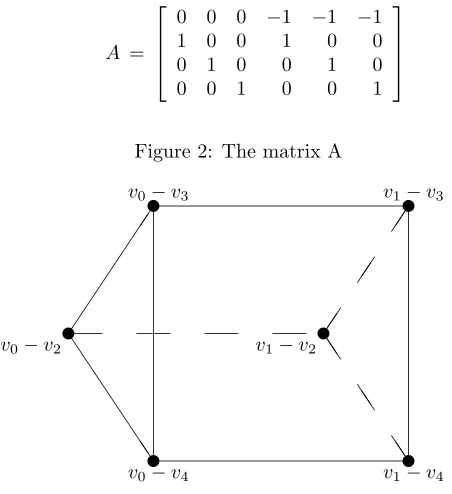
LetA= [a1, . . . , an] be ad×n-integer matrix whosed×d-minors are relatively
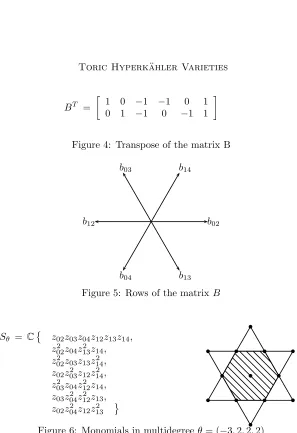
prime. We choose an n×(n−d)-matrix B = [b1, . . . , bn]T which makes the
following sequence exact:
0 −→ Zn−d −→B Zn −→A Zd −→ 0. (1) The choice of B is equivalent to choosing a basis in ker(A). The configura-tion B := {b1, . . . , bn} in Zn−d is said to be a Gale dual of the given vector
configuration A:={a1, . . . , an} inZd.
We denote byTC the complex groupC∗ and byTRthe circleU(1). Their Lie
algebras are denoted by tC and tR respectively. We apply the contravariant
functor Hom(·,TC) to the short exact sequence (1). This gives a short exact
sequence of abelian groups:
1 ←− TnC−d ←−BT TnC ←−AT TdC ←− 1. (2) ThusTd
C is embedded as ad-dimensional subtorus of TnC. It acts on the affine
space Cn. We shall construct the quotients of this action in the sense of ge-ometric invariant theory (= GIT). The ring of polynomial functions on Cn is
graded by the semigroupNA ⊆Zd:
S = C[x1, . . . , xn], deg(xi) = ai ∈ NA. (3)
A polynomial in S is homogeneous if and only if it is a Td
C-eigenvector. For
θ ∈ NA, let Sθ denote the (typically infinite-dimensional) C-vector space of
homogeneous polynomials of degree θ. Note that Sθ is a module over the
subalgebra S0 of degree zero polynomials in S = L
θ∈NASθ. The following
Lemma 2.1 The C-algebraS0 is generated by a finite set of monomials, cor-responding to the minimal generators of the semigroup Nn∩im(B). For any
θ ∈NA, the graded component Sθ is a finitely generated S0-module, and the ring S(θ) = L∞r=0Srθ is a finitely generated S0-algebra.
The C-algebra S0 coincides with the ring of invariants STd
C. The S0-algebra S(θ)is isomorphic toL∞r=0 trSrθ. We regard it asN-graded by the degree oft.
Definition 2.2 Theaffine GIT quotientof Cn by thed-torus TdC is the affine toric variety
X(A,0) := Cn//0TdC := Spec (STdC) = Spec (S0) = Spec¡C[Nn
∩im(B)]¢ . (4)
For any θ∈NA, theprojective GIT quotient of Cn by thed-torus Td C is the toric variety
X(A, θ) := Cn//θTdC := Proj (S(θ)) = Proj ∞
M
r=0 tr·S
rθ. (5)
Recall that the isomorphism class of any toric variety is given by a fan in a lattice. A toric variety is atoric orbifoldif its fan is simplicial. We shall describe the fans of the toric varietiesX(A,0) andX(A, θ) using the notation in Fulton’s book [8]. We writeM for the lattice Zn−d in (1) and N = Hom(M,Z) for its dual. The torus TnC−d in (2) is identified with N⊗ TC. The column vectors B ={b1, . . . , bn} of the matrix BT form a configuration in N ≃ Zn−d. We
write pos(B) for the convex polyhedral cone spanned byBin the vector space NR = N⊗ R ≃ Rn−d. Note that the affine toric variety associated with the
cone pos(B) equals X(A,0).
Atriangulationof the configurationBis a simplicial fan Σ whose rays lie inB
and whose support equals pos(B). A T-Cartier divisor on Σ is a continuous function Ψ : pos(B)→R which is linear on each cone of Σ and takes integer values on N∩pos(B). The triangulation Σ is called regular if there exists a T-Cartier divisor Ψ which isample, i.e. the function Ψ : pos(B)→R is convex and restricts to a different linear function on each maximal cone of Σ. Two T-Cartier divisors Ψ1 and Ψ2 are equivalent if Ψ1−Ψ2 is a linear map on pos(B), i.e. it is an element of M. A divisoron Σ is an equivalence class of T-Cartier divisors on Σ. Since Ψ1is ample if and only if Ψ2is ample, ampleness is well-defined for divisors [Ψ]. Finally, we define apolarized triangulationofB
to be a pair consisting of a triangulation Σ ofBand an ample divisor [Ψ]. The cokernel of M −→B Zn is identified withZdin (1) and we call it thePicard group. HenceA={a1, . . . , an} is a vector configuration in the Picard group. Thechamber complexΓ(A) ofAis defined to be the coarsest fan with support pos(A) that refines all triangulations ofA. Experts in toric geometry will note that Γ(A) equals the secondary fan of B as in [7]. We say that θ ∈ NA is
not in any lower-dimensional cone pos{ai1, . . . , aid−1} spanned by columns of
A. The chamber complex Γ(A) parameterizes the different combinatorial types of the convex polyhedra
Pθ =
©
u ∈ Rn : Au=θ, u≥0ª
as θ ranges over NA. In particular, θ is generic if and only if Pθ is (n−
d)-dimensional and each of its vertices has exactlydnon-zero coordinates (i.e.Pθ
is simple). A vector θin NAis called anintegral degreeif every vertex of the polyhedron Pθ is a lattice point inZn.
Proposition 2.3 There is a one-to-one correspondence between generic inte-gral degreesθinNAand polarized triangulations¡
Σ,[Ψ]¢
ofB. When forgetting the polarization this correspondence gives a bijection between open chambers of
Γ(A)and regular triangulations Σof B.
Proof: Given a generic integral degree θ, we construct the corresponding polarized triangulation ¡
Σ,[Ψ]¢
. First choose anyψ∈Znsuch thatAψ=−θ.
Then consider the polyhedron Qψ :=
©
v∈MR : Bv ≥ ψ
ª .
The map v 7→ Bv −ψ is an affine-linear isomorphism from Qψ onto Pθ
which identifies the set of lattice points Qψ ∩M with the set of lattice points
Pθ ∩ Zn. The set of linear functionals which are bounded below on Qψ is
precisely the cone pos(B)⊂N. Finally, define the function Ψ : pos(B)→R, w 7→ min{w·v : v∈Qψ}.
This is the support function ofQψ, which is piecewise-linear, convex and
con-tinuous. It takes integer values on N∩pos(B) because each vertex ofQψlies in
M. SinceQψ is a simple polyhedron, its normal fanis a regular triangulation
Σθ ofB, and Ψ restricts to a different linear function on each maximal face of
Σθ. Hence
¡ Σθ,[Ψ]
¢
is a polarized triangulation ofB. Conversely, if we are given a polarized triangulation ¡
Σ,[Ψ]¢
of B, then we define ψ := (Ψ(b1), . . . ,Ψ(bn)) ∈ Zn, and θ = −Aψ is the corresponding
generic integral degree inNA. ¤
Theorem 2.4 Let θ ∈ NA be a generic integral degree. Then X(A, θ) is an orbifold and equals the toric variety X(Σθ), whereΣθ is the regular triangula-tion of Bgiven by θas in Proposition 2.3.
Proof: First note that the multigraded polynomial ringSis thehomogeneous coordinate ringin the sense of Cox [6] of the toric varietyX(Σθ). Specifically,
L∞
r=1Srθ. Since Σθ is a simplicial fan, by [6, Theorem 2.1], X(Σθ) is the
geometric quotient ofCn\V(BΣ
θ) modulo T
d
C. The variety V(BΣθ) consists of
the points inCn which are not semi-stable with respect to theTd
C-action. By
standard results in Geometric Invariant Theory, the geometric quotient of the semi-stable locus in Cn modulo TdC coincides with X(A, θ) = Proj (S(θ)) =
Cn//
θTdC. Therefore X(A, θ) is isomorphic toX(Σθ). ¤
Corollary 2.5 The distinct GIT quotients X(A, θ) = Cn//θTdC which are toric orbifolds are in bijection with the open chambers inΓ(A), and hence with the regular triangulations ofB.
Recall that for every schemeX there is a canonical morphism
πX:X7→X0 (6)
to the affine scheme X0 = Spec(H0(X,OX)) of regular functions on X. We call a toric varietyX semi-projectiveifXhas at least one torus-fixed point and the morphismπX is projective.
Theorem 2.6 The following three classes of toric varieties coincide: 1. semi-projective toric orbifolds,
2. the GIT-quotients X(A, θ) constructed in(5)whereθ∈NA is a generic integral degree,
3. toric varieties X(Σ) where Σis a regular triangulation of a setB which spans the latticeN.
Proof: The equivalence of the classes 2 and 3 follows from Theorem 2.4. Let X(Σ) be a toric variety in class 3. Since B spans the lattice, the fan Σ has a full-dimensional cone, and hence X(Σ) has a torus-fixed point. Since Σ is simplicial, X(Σ) is an orbifold. The morphism πX can be described as
follows. The ring of global sections H0(X(Σ),OX(Σ)) is the semigroup algebra of the semigroup inM consisting of all linear functionals onN which are non-negative on the support|Σ|of Σ. Its spectrum is the affine toric variety whose cone is |Σ|. The triangulation Σ supports an ample T-Cartier divisor Ψ. The morphismπX is projective since it is induced by Ψ. HenceX(Σ) is in class 1.
Finally, letX be any semi-projective toric orbifold. It is represented by a fan Σ in a latticeN. The fan Σ is simplicial since X is an orbifold, and|Σ|spans NRsinceX has at least one fixed point. Since the morphismπX is projective,
the fan Σ is a regular triangulation of a subsetB′ of|Σ|which includes the rays
of Σ. The set B′ need not span the latticeN. We choose any supersetBofB′
which is contained in pos(B′) =|Σ| and which spans the latticeN. Then Σ
can also be regarded as a regular triangulation of B, and we conclude thatX
Remark. 1. The passage fromB′ to B in the last step means that any GIT
quotient of Cn′
modulo any abelian subgroup of Tn′
C can be rewritten as a
GIT quotient of some bigger affine space Cn modulo a subtorus of Tn C. This
construction applies in particular when the given abelian group is finite, in which case the initial subsetB′ ofN is linearly independent.
2. Our proof can be extended to show the following: if X is any toric variety where the morphismπXis projective thenXis the product of a semi-projective
toric variety and a torus.
3. The affinization map (6) forX(A, θ) is the canonical map toX(A,0). A triangulation Σ of a subset B of N ≃ Zn−d is called unimodular if every maximal cone of Σ is spanned by a basis ofN. This property holds if and only if X(Σ) is a toric manifold (= smooth toric variety). We say that a vector θ in NA is a smooth degree if C−1·θ ≥ 0 implies det(C) = ±1 for every non-singulard×d-submatrixCofA. Equivalently, the edges at any vertex of the polyhedronPθgenerate kerZA∼=Zn−d. From Theorem 2.6 we conclude:
Corollary 2.7 The following three classes of smooth toric varieties coincide: 1. semi-projective toric manifolds,
2. the GIT-quotients X(A, θ) constructed in(5)whereθ∈NA is a generic smooth degree,
3. toric varietiesX(Σ) where Σis a regular unimodular triangulation of a spanning setB ⊂N.
Definition 2.8 The matrixAis calledunimodularif the following equivalent conditions hold:
• all non-zerod×d-minors ofA have the same absolute value,
• all (n−d)×(n−d)-minors of the matrixB in (1) are−1,0 or+1, • every triangulation ofBis unimodular,
• every vectorθ inNAis an integral degree,
• every vectorθ inNAis a smooth degree.
Corollary 2.9 For A unimodular, every GIT quotient X(A, θ) is a semi-projective toric manifold, and the distinct smooth quotients X(A, θ)are in bi-jection with the open chambers inΓ(A).
2.1 is generated by a set of m+ 1 monomials in Sθ, possibly after replacing
θ by a multiple in the non-unimodular case. Let Pm
C be the projective space
whose coordinates are these monomials. Then, by definition of “Proj”, the toric varietyX(A, θ) is embedded as a closed subscheme in the product Pm
C ×
Spec(S0). We have an action of the (n−d)-torus TnC/Td
C onPmC, sinceSθ is
an eigenspace of TdC. This gives rise to a moment map µ1 : PmC → Rn−d, whose image is a convex polytope. Likewise, we have the affine moment map µ2 : Spec(S0)→Rn−d whose image is the cone polar to pos(B). This defines the moment map
µ : X(A, θ) ⊂ PmC ×Spec(S0) → Rn−d, (u, v)7→µ1(u) +µ2(v). (7) The image of X(A, θ) under the moment map µis the polyhedronPθ ≃ Qψ,
since the convex hull of its vertices equals the image ofµ1and the coneP0≃Q0 equals the image ofµ2.
Given an arbitrary fan Σ inN, Section 2.3 in [8] describes how a one-parameter subgroup λv, given by v ∈N, acts on the toric variety X(Σ). Consider any
pointxin X(Σ) and letγ∈Σ be the unique cone such that xlies in the orbit Oγ. The orbitOγ is fixed pointwise by the one-parameter subgroupλv if and
only if v lies in the R-linear span Rγ of γ. Thus the irreducible components Fi of the fixed point locus of the λv-action on X(Σ) are the orbit closures
Oσi where σi runs over all cones in Σ which are minimal with respect to the
property v∈Rσi.
The closure ofOγinX(Σ) is the toric varietyX(Star(γ)) given by the quotient
fan Star(γ) in N(γ) =N/(N∩Rγ); see [8, page 52]. From this we can derive the following lemma.
Lemma 2.10 Forv ∈N andx∈Oγ the limit limz→0λv(z)x exists and lies in Fi =Oσi if and only if γ⊆σi is a face and the image ofv in NR/Rγ is in
the relative interior of σi/Rγ.
The set of all facesγofσiwith this property is closed under taking intersections
and hence this set has a unique minimal element. We denote this minimal element byτi. Thus if we denote
Uiv =
©
x∈X(Σ) : lim
z→0λv(z)x exists and lies inFi ª
,
or justUi for short, then this set decomposes as a union of orbits as follows:
Ui = ∪τi⊆γ⊆σiOγ. (8)
In what follows we further supposev∈ |Σ|. Then Lemma 2.10 impliesX(Σ) =
∪iUi, which is theBialynicki-Birula decomposition[2] of the toric variety with
respect to the one-parameter subgroupλv.
We now apply this to our semi-projective toric varietyX(A, θ) with fan Σ = Σθ.
product µv(x) =hv, µ(x)iwith µas in (7). We relabel the fixed components
Fi according to the values of this moment map, so that
µv(Fi)< µv(Fj) impliesi < j. (9)
Given this labeling, the distinguished facesτi⊆σihave the following important
property:
τi⊆σj implies i≤j. (10)
This generalizes the property (∗) in [8, Chapter 5.2], and it is equivalent to Uj is closed in U≤j =∪i≤jUi. (11)
This means that the Bialynicki-Birula decomposition of X(A, θ) is filtrablein the sense of [2]. The following is well-known in the projective case.
Proposition 2.11 The integral cohomology of a smooth semi-projective toric variety X(A, θ)equals
H∗(X(A, θ);Z) ∼= Z[x1, x2, . . . , xn]/(Circ(A) +Iθ),
where Iθ is the Stanley-Reisner ideal of the simplicial fan Σθ, i.e. Iθ is generated by square-free monomials xi1xi2· · ·xik corresponding to non-faces
{bi1, bi2, . . ., bik} of Σθ, andCirc(A) is thecircuit ideal
Circ(A) := h n
X
i=1
λixi |λ∈Zn, A·λ= 0i.
Proof: Let D1, D2, . . . , Dn denote the divisors corresponding to the rays
b1, b2, . . . , bn in Σθ. The cohomology class of any torus orbit closure Oσ can
be expressed in terms of the Di’s, namely if the rays in σare bi1, bi2, . . . , bik,
then [Oσ] = [Di1][Di2]· · ·[Dik]. Following the reasoning in [8, Section 5.2], we
first prove that certain torus orbit closures linearly span H∗(X(A, θ);Z) and
hence the cohomology classes [D1],[D2], . . . ,[Dn] generateH∗(X(A, θ);Z) as a
Z-algebra.
We choose v ∈ |Σ| to be generic, so that each σi is (n−d)-dimensional and
eachFi is just a point. Then (8) shows thatUi is isomorphic with the affine
spaceCn−ki, wherek
i= dim(τi).
We set U≤j = ∪i≤jUi and U<j = ∪i<jUi. Note that Uj is closed in U≤j.
Thus writing down the cohomology long exact sequence of the pair (U≤j, U<j),
we can show by induction on j that the cohomology classes of the closures of the cells Ui generate H∗(X(A, θ);Z) additively. Because the closure of a
cell Ui is the closure of a torus orbit, it follows that the cohomology classes
[D1],[D2], . . . ,[Dn] generate H∗(X(A, θ);Z). Thus sendingxi 7→[Di] defines
to contain Circ(A) +Iθ. That this is precisely the kernel follows from the
“algebraic moving lemma” of [8, page 107]. ¤
A similar proof works withQ-coefficients whenX(A, θ) is not smooth but just an orbifold.
Corollary 2.12 The rational cohomology ring of a semi-projective toric orb-ifold X(A, θ) equals
H∗(X(A, θ);Q) ∼= Q[u1, u2, . . . , un]/(Circ(A) +Iθ).
In light of Corollary 2.12, the Betti numbers of X(A, θ) satisfy b2i =hi(Σθ),
wherehi(Σθ) are theh-numbers of the Stanley-Reisner idealIθ, cf. [18, Section
III.3]. This observation leads to the following result.
Corollary 2.13 If fi(Pθbd) denotes the number of i-dimensional bounded faces ofPθ then the Betti numbers of the semi-projective toric orbifoldX(A, θ) are given by the following formula:
b2k = dimQH2k(X(A, θ);Q) = n−d
X
i=k
(−1)i−k
¡
ki¢
fi(Pθbd). (12)Proof: Lemma 2.3 of [19] implies that
n−d
X
i=0
hi(Σθ)·xi =
X
σ∈Σθ\∂Σθ
(x−1)n−d−dim(σ), (13)
where ∂Σθ denotes the boundary of Σθ. Hence the right hand sum is over all
interior conesσof the fan Σθ. These cones are in order-reversing bijection with
the bounded faces ofPθ. Hence (13) is the sum of (x−1)dim(F) whereF runs
over all bounded faces ofPθ. This proves (12). ¤
3 The core of a toric variety
The proof of Corollary 2.13 shows the importance of interior cones of Σθ. They
are the ones for which the closure of the corresponding torus orbit in X(A, θ) is compact. This suggests the following
Definition 3.1 The core of a semi-projective toric variety X(A, θ) is
C(A, θ) = ∪σ∈Σθ\∂ΣθOσ. Thus the core C(A, θ) is the union of all compact
torus orbit closures in X(A, θ).
Theorem 3.2 The core of a semi-projective toric orbifoldX(A, θ) is the in-verse image of the origin under the canonical projective morphism X(A, θ)→
Proof: On the level of fans, the toric morphism X(A, θ)→ X(A,0) corre-sponds to forgetting the triangulation of the cone |Σ|= pos(B). It follows from the description of toric morphisms in Section 1.4 of [8] that the inverse image of the origin is the union of the orbit closures corresponding to interior faces of Σ. This was our first assertion. Each face of a simple polyhedron is a simple polyhedron, and each bounded face is a simple polytope. If σ is the interior cone of Σ dual to a bounded face ofPθ then the corresponding orbit closure is
the projective toric orbifoldX(Star(σ)). The coreC(A, θ) is the union of these
orbifolds. ¤
We fix a generic vector v ∈ int|Σ|. Then the Fi above are points and lie
in C(A, θ). In what follows we shall study the action of the one-parameter subgroupλv on the coreC(A, θ). We define
Di = Ui−v =
©
x∈X(A, θ) : lim
z→∞λv(z)x exists and equalsFi
ª .
Lemma 2.10 implies that this gives a decomposition of the core: C(A, θ) =
∪iDi. The closure Di is a projective toric orbifold, and it is the preimage of a
bounded face ofPθ via the moment map (7). If we now introduce an ordering
as in (9) then the counterpart of (11) is the following:
D≤j = ∪i≤jDi is compact. (14)
This property of the decomposition C(A, θ) = ∪iDi translates into a
non-trivial statement about the convex polyhedronPθ. LetPθbddenote thebounded complex, that is, the polyhedral complex consisting of all bounded faces ofPθ.
LetPj denote the bounded face of Pθ corresponding toDj, and letpj denote
the vertex ofPθ corresponding toFj. Then P≤j = ∪i≤jPi is a subcomplex
of the bounded complexPbd
θ , and P≤j\P<j consists precisely of those faces of
Pj which contain pj. This property is calledstar-collapsibility. It implies that
P<j is a deformation retract ofP≤j and in turn thatPθbd is contractible. The
contractibility also follows from [4, Exercise 4.27 (a)]. In summary we have proven the following result.
Theorem 3.3 The bounded complexPbd
θ ofPθis star-collapsible; in particular, it is contractible.
This theorem implies that the core of any semi-projective toric variety is con-nected, since C(A, θ) is the preimage of the bounded complex Pbd
θ under the
continuous moment map. Moreover, since the cohomology ofPbd
θ vanishes, the
Proof: Letv∈int|Σ|,Fi andDi as above. We prove by induction on j that
ifα∈H∗(D≤j;Q) andα|Di= 0 fori≤j, thenα= 0. (15)
This implies the proposition, because if α vanishes on every irreducible com-ponent of the core then it vanishes on every irreducible projective subvariety Di of the core. The statement (15) then implies by induction that αvanishes
on the core.
To prove (15) consider the Mayer-Vietoris sequence of the covering D≤j =
D<j∪Dj.
. . .→Hk(D
≤j;Q)→α Hk(D<j;Q)⊕Hk(Dj;Q) β →Hk(D
<j∩Dj;Q)→. . .
We show that the map αis injective, which will prove our claim. For this we show that β is surjective. This follows from the surjectivity of Hk(D
j;Q)→
Hk(Dj\D
j;Q), because clearlyD<j∩Dj=Dj\Dj.
To prove this we do Morse theory on the projective toric orbifoldDj. First it
follows from Morse theory thatH∗(D
j;Q)→H∗(Dj\Fj;Q) surjects. Moreover
we have that Dj\Dj is the core of the quasi-projective variety Dj\Fj. This
means thatDj\Dj is the set of pointsxinDj such that limz→∞λv(z)xis not
in Fj. Then the proof of Theorem 3.5 shows that H∗(Dj\Fj;Q) is isomorphic
withH∗(D
j\Dj;Q). This proves (15) and in turn our Proposition 3.4. ¤
We finish this section with an explicit description of the cohomology ring of C(A, θ), namely, we identify it with the cohomology of the ambient semi-projective toric orbifold X(A, θ):
Theorem 3.5 The embedding of the core C(A, θ)in X(A, θ) induces an iso-morphism on cohomology with integer coefficients.
Proof: Let v ∈ int|Σ|, Fi, Ui and Di as above. We clearly have an
inclu-sion D≤j ⊂ U≤j. We show by induction on j that this inclusion induces an
isomorphism on cohomology. Consider the following commutative diagram: . . .→ Hk(U
≤j, U<j;Z) → Hk(U≤j;Z) → Hk(U<j;Z) →. . .
↓ ↓ ↓
. . .→ Hk(D
≤j, D<j;Z) → Hk(D≤j;Z) → Hk(D<j;Z) →. . .
.
The rows are the long exact sequence of the pairs (U≤j, U<j) and (D≤j, D<j)
respectively. The vertical arrows are induced by inclusion. The last vertical arrow is an isomorphism by induction.
By excisionHk(U
≤j, U<j;Z)∼=Hk(T(Nj), t0;Z), whereNjis the normal
(orbi-)bundle to Uj and T(Nj) is the Thom space Nj∪t0, where t0 is the point
at infinity. Similarly Hk(D
≤j, D<j;Z) ∼= Hk(T(Dj), t0;Z), where T(Dj) =
D≤j/D<j is the one point compactification of Dj, which is homeomorphic
to the Thom space of Nj|Fj, the negative bundle at Fj. Because Fj is a
restricts to the normal bundle ofFjinDj, we find thatT(Dj) is a deformation
retract ofT(Nj). Consequently the first vertical arrow is also an isomorphism.
The Five Lemma now delivers our assertion. ¤
Remark. One can prove more, namely, thatC(A, θ) is a deformation retract ofX(A, θ). This follows from Theorem 3.5 and the analogous statement about the fundamental group, which vanishes for both spaces. Alternatively, one can use Bott-Morse theory in the spirit of the proof of [16, Theorem 3.2] to get the homotopy equivalence.
4 Lawrence toric varieties
In this section we examine an important class of toric varieties which are semi-projective but not semi-projective. We fix an integerd×n-matrixAas in (1), and we writeA± = [A,−A] for thed×2n-matrix obtained by appending the negative
ofAtoA. The corresponding vector configuration A± =A ∪ −A spansZdas
a semigroup; in symbols, NA±=ZA=Zd. A vectorθisgenericwith respect
toA± if it does not lie on any hyperplane spanned by a subset ofA.
Definition 4.1 We call X(A±, θ) a Lawrence toric variety, for any generic vectorθ∈Zd.
Our choice of name comes from the Lawrence construction in polytope theory; see e.g. Chapter 6 in [22]. The Gale dual of the centrally symmetric configu-ration A± is denoted Λ(B) and is called theLawrence liftingof B. It consists
of 2n vectors which span Z2n−d. The cone pos(Λ(B)) is the cone over the
(2n−d−1)-dimensionalLawrence polytopewith Gale transformA±.
Consider the even-dimensional affine space C2n with coordinates
z1, . . . , zn, w1, . . . , wn. We call a torus action on C2n symplectic if the
products z1w1, . . . , znwn are fixed under this action.
Proposition 4.2 The following three classes of toric varieties coincide: 1. Lawrence toric varieties,
2. toric orbifolds which are GIT-quotients of a symplectic torus action on
C2n for somen∈N,
3. toric varietiesX(Σ) whereΣ is the cone over a regular triangulation of a Lawrence polytope.
Proof: This follows from Theorem 2.6 using the observation that a torus action on C2n is symplectic if and only if it arises from a matrix of the form A±. This means the action looks like
Note that a polytope is Lawrence if and only if its Gale transform is centrally
symmetric. ¤
The matrixA±is unimodular if and only if the smaller matrixAis unimodular.
Therefore unimodularity of A implies the smoothness of the Lawrence toric variety, by Corollary 2.9. An interesting feature of Lawrence toric varieties is that the converse to this statement also holds:
Proposition 4.3 The Lawrence toric varietyX(A±, θ) is smooth if and only if Ais unimodular.
Proof: The chamber complex Γ(A±) is the arrangement of hyperplanes
spanned by subsets of A. The vector θ is assumed to lie in an open cell of that arrangement. For any column basisC={ai1, . . . , aid}of thed×n-matrix
A there exists a unique linear combination
λ1ai1 + λ2ai2 +· · · + λdaid = θ.
Here all the coefficients λj are non-zero rational numbers. We consider the
polynomial ring
Z[x, y] = Z[x1, . . . , xn, y1, . . . , yn].
The 2n variables are used to index the elements of A± and the elements of
Λ(B). We set
σ(C, θ) = {xij : λj >0} ∪ {yij : λj<0}.
Its complement σ(C, θ) = ©
x1, . . . , xn, y1, . . . , ynª\σ(C, θ) corresponds to a
subset of Λ(B) which forms a basis of R2n−d. The triangulation Σ
θ of the
Lawrence polytope defined byθis identified with its set of maximal faces. This set equals
Σθ = ©σ(C, θ) : C is any column basis ofAª. (16)
Hence the Lawrence toric variety X(A±, θ) = X(Σ
θ) is smooth if and only if
every basis in Λ(B) spans the lattice Z2n−d if and only if every column basis
C of A spans Zd. The latter condition is equivalent to saying that A is a
unimodular matrix. ¤
Corollary 4.4 The Stanley-Reisner ideal of the fanΣθ equals
Iθ =
\
C
hσ(C, θ)i ⊂ Z[x, y], (17)
i.e. Iθ is the intersection of the monomial prime ideals generated by the sets
σ(C, θ) where C runs over all column bases of A. The irrelevant ideal of the Lawrence toric variety X(Σθ)equals
Bθ = h
Y
We now compute the cohomology of a Lawrence toric variety. For simplicity of exposition we assume A is unimodular so that X(A±, θ) is smooth. The
orbifold case is analogous. First note
Circ(A±) = hx1+y1, x2+y2, . . . , xn+xni + Circ(A),
where Circ(A) is generated by all linear forms Pn
i=1λixi such that λ =
(λ1, . . . , λn) lies in ker(A) = im(B). From Proposition 2.11, we have
H∗¡
X(A±, θ) =Z[x, y]/ µ
hx1+y1, x2+y2, . . . , xn+yni + Circ(A) + Iθ
¶ .
Letφdenote theZ-algebra epimorphism which collapses the variables pairwise: φ : Z[x1, . . . , xn, y1, . . . , yn] → Z[x1, . . . , xn], xi7→xi, yi7→ −xi.
Then we can rewrite the presentation of the cohomology ring as follows:
H∗¡
X(A±, θ);Z¢
= Z[x1, . . . , xn]/
µ
Circ(A) + φ(Iθ)
¶ .
Clearly, the image of the ideal (17) underφis the intersection of the ideals φ¡
hσ(C, θ)i¢
= hxi: i∈Ci
whereC runs over the column bases ofA. Note that this ideal is independent of the choice ofθ. It depends only onA. This ideal is called thematroid ideal
ofBand it is abbreviated by
M∗(A) = \©hxi1, . . . , xidi : {ai1, . . . , aid} ⊆ A is linearly independent
ª = hxi1· · ·xik :{bi1, . . . , bik} ⊆ B is linearly dependenti
= M(B).
We summarize what we have proven concerning the cohomology of a Lawrence toric variety.
Theorem 4.5 The integral cohomology ring of a smooth Lawrence toric variety
X(A±, θ) is independent of the choice of the generic vectorθ inZd. It equals
H∗¡
X(A±, θ);Z¢
= Z[x1, . . . , xn]/¡Circ(A) + M∗(A)¢. (19) The same holds for Lawrence toric orbifolds with Zreplaced byQ.
The ring Q[x1, . . . , xn]/M∗(A) is the Stanley-Reisner ring of the matroid
com-plex (of linearly independent subsets) of the (n−d)-dimensional configuration
B. This ring is Cohen-Macaulay, and Circ(A) provides a linear system of parameters. We write h(B) = (h0, h1, . . . , hn−d) for its h-vector. This is a
well-studied quantity in combinatorics; see e.g. [5] and [18, Section III.3]. Corollary 4.6 The Betti numbers of the Lawrence toric variety X(A±, θ) are independent of θ, and they coincide with the entries in the h-vector of the rank n−dmatroid given byB:
dimQH2i(X(A±, θ);Q) = hi(B). for i= 0,1, . . . , n−d.
Our second result in this section concerns the core of a Lawrence toric variety of dimension 2n−d. We fix a generic vectorθinZd. The fan Σ
θis the normal
fan of the unbounded polyhedron
Pθ = ©(u, v)∈Rn⊕Rn : Au−Av = θ, u, v≥0ª.
As in the proof of Proposition 2.3, we chose any vectorψ∈Znsuch that Aψ =
−θ, and we consider the following full-dimensional unbounded polyhedron in R2n−d:
Qψ =
©
(w, t)∈Rn−d⊕Rn : t ≥ 0, Bw +t ≥ ψª .
The map (w, t)7→(Bw+t−ψ, t) is an affine-linear isomorphism fromQψonto
Pθ. We defineH(B, ψ) to be the arrangement of the following nhyperplanes
in Rn−d:
{w∈Rn−d : bi·w=ψi} (i= 1,2, . . . , n).
The arrangementH(B, ψ) is regarded as a polyhedral subdivision ofRn−dinto relatively open polyhedra of various dimensions. The collection of all such polyhedra which are bounded form a subcomplex, called the bounded complex
ofH(B, ψ) and denoted byHbd(B, ψ).
Theorem 4.7 The bounded complexHbd(B, ψ)of the hyperplane arrangement H(B, ψ)inRn−d is isomorphic to the complex of bounded faces of the(2n−d) -dimensional polyhedron Qψ≃Pθ.
Proof: We define an injective map from Rn−d into the polyhedron Q ψ as
follows
w 7→ ¡ w, t¢
, where ti = max{0, ψi−bi·w}. (20)
This map is linear on each cell of the hyperplane arrangementH(B, ψ), and the image of each cell is a face ofQψ. In particular, every bounded cell ofH(B, ψ)
is mapped to a bounded face of Qψ and each unbounded cell of H(B, ψ) is
mapped to an unbounded face of Qψ. It remains to be shown that every
Now, the image of (20) is the following subcomplex in the boundary of our polyhedron:
{(w, t)∈Qψ : ti·(bi·w+ti−ψi) = 0 fori= 1,2, . . . , n
ª
≃ {(u, v)∈Pθ : ui·vi= 0 fori= 1,2, . . . , n
ª
Consider any face F of Pθ which is not in this subcomplex, and let (u, v) be
a point in the relative interior of F. There exists an indexi with ui >0 and
vi >0. Let ei denote the i-th unit vector in Rn. For every positive realλ,
the vector (u+λei, v+λei) lies in Pθ and has the support as (u, v). Hence
(u+λei, v+λei) lies inF for allλ≥0. This shows thatF is unbounded. ¤
Theorem 4.7 and Corollary 2.13 imply the following enumerative result: Corollary 4.8 The Betti numbers of the Lawrence toric variety X(A±, θ) satisfy
dimQH2i(X(A±, θ);Q) = n−d
X
i=k
(−1)i−k
¡
ki¢
fi(Hbd(B, ψ)),where fi(Hbd(B, ψ)) denotes the number of i-dimensional bounded regions in H(B, ψ).
There are two natural geometric structures on any Lawrence toric variety. First the canonical bundle of X(A±, θ) is trivial, because the vectors in A± add
to 0. This means that X(A±, θ) is a Calabi-Yau variety. Moreover, since
the symplectic TdC-action preserves the natural Poisson structure on C2n ∼= Cn⊕(Cn)∗, the GIT quotientX(A±, θ) inherits a naturalholomorphic Poisson structure. The holomorphic symplectic leaves of this Poisson structure are what we call toric hyperk¨ahler manifolds. The special leaf which contains the core of X(A±, θ) will be called the toric hyperk¨ahler variety. We present these
definitions in complete detail in the following two sections.
5 Hyperk¨ahler quotients
Our aim is to describe an algebraic approach to the toric hyperk¨ahler manifolds of Bielawski and Dancer [3]. In this section we sketch the original differential geometric construction in [3]. This construction is the hyperk¨ahler analogue to the construction of toric varieties using K¨ahler quotients. We first briefly review the latter. Fix the standard Euclidean bilinear form onCn,
g(z, w) =
n
X
i=1
(re(zi)re(wi) + im(zi)im(wi)).
The correspondingK¨ahler form is
ω(z, w) = g(iz, w) =
n
X
i=1
LetAbe as in (1) and consider the real torusTd
Rwhich is the maximal compact
subgroup of Td
C. The group TdR acts on Cn preserving the K¨ahler structure.
This action has the moment map
µR : Cn → (tdR)
Zdthen there is a biholomorphism between the smooth loci in the GIT quotient X(A, θ) and the K¨ahler quotientX(A, ξR). Hence if A is unimodular and θ
generic then the complex manifoldsX(A, θ) andX(A, ξR) are biholomorphic.
Now we turn to toric hyperk¨ahler manifolds. LetHbe the skew field of quater-nions, the 4-dimensional real vector space with basis 1, i, j, k and associative algebra structure given by i2 = j2 =k2 =ijk =−1. Left multiplication by i (resp. j and k) defines complex structures I : H → H, with I2 = −Id
H,
(resp. J andK) on H. We now put the flat metric g on Harising from the standard Euclidean scalar product onH∼=R4 with 1, i, j, k as an orthonormal basis. This is called a hyperk¨ahler metric because it is a K¨ahler metric with respect to all three complex structuresI, J and K. It means that the differ-ential 2-forms, the so-called K¨ahler forms, given byωI(X, Y) =g(IX, Y) for
tangent vectors X andY, and the analogously definedωJ andωK are closed.
For the reader’s convenience we write down these K¨ahler forms in coordinates (x, y, u, v):
ωI =dx∧dy+du∧dv,
ωJ =dx∧du+dv∧dy,
ωK=dx∧dv+dy∧du.
A special orthogonal transformation, with respect to this metric, is said to pre-serve the hyperk¨ahler structure if it commutes with all three complex structures I,J andKor equivalently if it preserves the K¨ahler formsωI,ωJandωK. The
group of such transformations, the unitary symplectic group Sp(1), is gener-ated by multiplication by unit quaternions from the right. A maximal abelian subgroupTR∼=U(1)⊂Sp(1) is thus specified by a choice of a unit quaternion.
We break the symmetry between I, J and K and choose the maximal torus generated by multiplication from the right by the unit quaternioni. ThusU(1) acts onHby sendingξtoξexp(φi), forexp(φi)∈U(1)⊂R⊕Ri∼=C. It follows from (21) that the moment map µI : H→ R with respect to the symplectic
form ωI is given by Similarly we obtain formulas for µJ and µK by writing down the eigenspace
=µJ
as the holomorphic moment map for theI-holomorphic action ofTC⊃TR on
H with respect to theI-holomorphic symplectic form ωC =ωJ +iωK. If we
identify Hwith C⊕Cby introducing two complex coordinates, z=x+iy ∈
R⊕Ri∼=C andw =v−ui∈R⊕Ri ∼=C, then the I-holomorphic moment mapµC:H→Cis given algebraically by multiplying complex numbers:
µC(z, w) = µJ(z, w) + iµK(z, w) = yu+xv +i(yv−xu) = zw. (23)
The discussion in the previous paragraph generalizes in an obvious man-ner to Hn for n > 1. Indeed, the n-dimensional quaternionic space Hn has three complex structures I,J and K, given by left multiplication with i, j, k ∈ H. Putting the flat metric gn = g⊕n on Hn yields a hyperk¨ahler
metric, i.e. the differential 2-forms ωI(X, Y) = gn(IX, Y) and similarly ωJ
and ωK are K¨ahler (meaning closed) forms. The automorphism group of
this hyperk¨ahler structure is the unitary symplectic groupSp(n). We fix the maximal torus Tn
R = U(1)n ⊂ Sp(n) given by the following definition. For
λ= (exp(φ1i),exp(φ2i), . . . ,exp(φni))∈TnRand (ξ1, ξ2, . . . , ξn)∈Hn we set
λ(ξ1, ξ2, . . . , ξn) = (ξ1exp(φ1i), ξ2exp(φ2i), . . . , ξnexp(φni)). (24)
As in the n= 1 case above, this fixes an isomorphism Hn ∼=Cn⊕Cn where
two complex vectors z, w ∈Cn ∼=Rn⊕iRn represent the quaternionic vector
z+wk ∈ Hn ∼= Rn⊕iRn⊕jRn⊕kRn. Expressing vectors in Hn in these
complex coordinates, the torus action (24) translates into
λ(z, w) = (λz, λ−1w) for λ∈TnR and (z, w)∈Hn. (25) The toric hyperk¨ahler manifolds in [3] are constructed by choosing a subtorus Td
R ⊂TnR and taking the hyperk¨ahler quotient [10] of Hn byTdR. We do this
by choosing integer matrices Aand B as in (1) and (2). The subtorusTd R of
Tn
R acts onHn by (25) preserving the hyperk¨ahler structure. Thehyperk¨ahler moment mapof the action (25) ofTd
ωK respectively. Using the formulas (22) and (23), the components ofµare in
µC(z, w) := µJ(z, w) +iµK(z, w) = n
X
i=1
ziwi·ai ∈ (tdR) ∗
⊗C∼= (tdC)∗. (27)
Here ai is thei-th column vector of the matrix A. We can also think of µC
as the moment map for theI-holomorphic action ofTdC onHn with respect to ωC=ωJ+iωK. Now take
ξ= (ξ1, ξ2, ξ3) ∈ (tdR)∗⊗R3
and introduce ξR = ξ1 ∈ (tdR)∗ and ξC = ξ2+iξ3 ∈ (tdC)∗ so we can write
ξ= (ξR, ξC)∈(tdR)∗⊕(tdC)∗. The hyperk¨ahler quotientofHn by the action (25)
of the torusTd
R at levelξis defined as
Y(A, ξ) := Hn////ξTRd := µ−1(ξ)/TdR =
¡
µ−R1(ξR)∩µ−C1(ξC)
¢
/TdR. (28)
By a theorem of [10], this quotient has a canonical hyperk¨ahler structure on its smooth locus.
Bielawski and Dancer show in [3] that ifξ∈(tdR)∗⊗R3 is generic thenY(A, ξ) is an orbifold, and it is smooth if and only if A is unimodular. Since ξ is generic outside a set of codimension three in (tdR)∗⊗R3, they can show that the topology and therefore the cohomology of the toric hyperk¨ahler manifold is independent onξ. In what follows we consider vectorsξfor whichξC= 0 inCd
and ξR=θ ∈Zd ⊂Rd ∼= (tdR)∗. The underlying complex manifold in complex
structure I of the hyperk¨ahler manifold Y(A,(θ,0C)) has a purely algebraic
description as explained in the next section.
6 Algebraic construction of toric hyperk¨ahler varieties The Zd-graded polynomial ring C[z, w] = C[z1, . . . , z
n, w1, . . . , wn], with the
grading given by A± = [A,−A], is the homogeneous coordinate ring of the
Lawrence toric variety X(A±, θ). By a result of Cox [6], closed subschemes
of X(A±, θ) correspond to homogeneous ideals inC[z, w] which are saturated
with respect to the irrelevant idealBθ in (18). Let us now consider the ideal
Circ(B) := h n
X
i=1
aijziwi |j= 1, . . . , di ⊂ C[z, w], (29)
whose generators are the components of the holomorphic moment map µC of
(27). The ideal Circ(B) is clearly homogeneous and it is a complete intersection. We assume that none of the row vectors of the matrix B is zero. Under this hypothesis, the ideal Circ(B) is a prime ideal.
Definition 6.1The toric hyperk¨ahler variety Y(A, θ) is the irreducible sub-variety of the Lawrence toric sub-varietyX(A, θ)defined by the homogeneous ideal
Proposition 6.2 If θ is generic then the toric hyperk¨ahler variety Y(A, θ)is an orbifold. It is smooth if and only if the matrixA is unimodular.
Proof: It follows from (27) that a point in C2n has a finite stabilizer under the group TdC if and only if the point is regular for µC of (27), i.e. if the
derivative of µC is surjective there. This implies that, forθ generic, the toric
hyperk¨ahler variety Y(A, θ) is an orbifold because then the varietyX(A±, θ)
is an orbifold. For the second statement note that if A is unimodular then X(A±, θ) is smooth, consequentlyY(A, θ) is also smooth. However, ifAis not
unimodular thenX(A±, θ) has orbifold singularities which lie in the core. Now
the core C(A±, θ) lies entirely inY(A, θ), by Lemma 6.4 below, thusY(A, θ)
inherits singular points fromX(A±, θ). ¤
We can now prove that our toric hyperk¨ahler varieties are biholomorphic to the toric hyperk¨ahler manifolds of the previous section.
Theorem 6.3 Let ξR = θ ∈ Zd ⊂ (tdR)∗ ∼=Rd for generic θ. Then the toric hyperk¨ahler manifold Y(A,(ξR,0)) with complex structure I is biholomorphic with the toric hyperk¨ahler varietyY(A, θ).
Proof: Suppose A is unimodular. The general theory of K¨ahler quotients (e.g. in [12]) implies that the Lawrence toric variety X(A±, θ) and the
corre-sponding K¨ahler quotientX(A±, ξ
R) =µ−R1(ξR)/TdRare biholomorphic, where
µR is defined in (26) and ξR = θ ∈Zd ⊂Rd ∼= (tdR)∗. Now the point is that
µC : Hn →Cd is invariant under the action of TdR and therefore descends to
a map on X(A±, ξR) = µR−1(ξR)/TdR and similarly on X(A
±, θ) making the
following diagram commutative:
µξC: X(A±, ξR) → Cd ∼
= ∼=
µθ
C: X(A±, θ) → Cd
.
It follows that Y(A,(ξR,0)) = (µξC)−1(0) and Y(A, θ) = (µθC)−1(0) are
biholo-morphic. The proof is similar when the spaces have orbifold singularities. ¤ Recall the affinization map πX : X(A±, θ) → X(A±,0) from (6), and the
analogous map πY : Y(A, θ) → Y(A,0). These fit together in the following
commutative diagram:
Y(A, θ) πY
→ Y(A,0) iθ↓ ↓i0
X(A±, θ) πX
→ X(A±,0)
µθ
C↓ ↓µ0C
Cd ∼= Cd ,
whereiθ:Y(A, θ)→X(A±, θ) denotes the natural embedding in Definition 6.1
by the preimage of µθ
Cat 0∈Cd. From this we deduce the following lemma:
Lemma 6.4 The cores of the Lawrence toric variety and of the toric hy-perk¨ahler variety coincide, that is, C(A±, θ) =π−1
X (0) =π −1
Remark. It is shown in [3] that the core of the toric hyperk¨ahler manifold Y(A, θ) is the preimage of the bounded complex in the hyperplane arrangement
H(B, ψ) by the hyperk¨ahler moment map. We know from Theorem 3.2 that the core of the Lawrence toric variety equals the preimage ofPbd
θ under the K¨ahler
moment map. Thus Theorem 4.7 is a combinatorial analogue of Lemma 6.4. We need one last ingredient in order to prove the theorem stated in the Intro-duction.
Lemma 6.5 The embedding of the coreC(A±, θ) in Y(A, θ)gives an isomor-phism in cohomology.
Proof: Consider theTC-action on the Lawrence toric varietyX(A±, θ) defined
by the vector v =Pn
i=1bi ∈Zn−d. This action comes from multiplication by
non-zero complex numbers on the vector spaceC2n. The holomorphic moment
map µC of (27) is homogeneous with respect to multiplication by a non-zero
complex number, and consequently µθ
C is also homogeneous with respect to
the circle actionλv. It follows that thisTC-action leaves the toric hyperk¨ahler
variety invariant. Moreover, since v is in the interior of pos(B), all the results in Section 3 are valid for this TC-action on X(A±, θ). Now the proof of
The-orem 3.5 can be repeated verbatim to show that the cohomology of Y(A, θ)
agrees with the cohomology of the core. ¤
Proof of Theorem 1.1: 1.= 3. is a consequence of Lemma 6.4 and Lemma 6.5.
2.= 3. This is a consequence of Theorem 3.5. 1.= 4. is the content of Theorem 4.5. ¤
Remark. 1. In fact, we could claim more than the isomorphism of cohomology rings in Theorem 1.1. The remark after Theorem 3.5 implies that the spaces C(A±, θ) ⊂Y(A, θ) ⊂X(A±, θ) are deformation retracts in one another. A
similar result appears in [3, Theorem 6.5].
2. The result 2.=4. in the smooth case was proven by Konno in [14].
3. We deduce from Theorem 1.1, Corollary 4.6 and Corollary 4.8 the following formulas for Betti numbers. The second formula is due to Bielawski and Dancer [3, Theorem 6.7].
Corollary 6.6 The Betti numbers of the toric hyperk¨ahler variety Y(A, θ)
agree with:
• theh-numbers of the matroid ofB: b2k(Y(A, θ)) = hk(B).
• the following linear combination of the number of bounded regions of the affine hyperplane arrangementH(B, ψ):
b2k(Y(A, θ)) = n−d
X
i=k
This corollary shows the importance of the combinatorics of the bounded com-plexHbd(B, ψ) in the topology ofY(A, θ) andX(A±, θ). This intriguing
con-nection will be more apparent in the next section. Before we get there we infer some important properties of the bounded complex from Corollary 9.1 and Theorem E of [21].
Proposition 6.7 The bounded complex Hbd(B, ψ) is pure-dimensional. Ifψ is generic and B is coloop-free then every maximal face of Hbd(B, ψ) is an
(n−d)-dimensional simple polytope.
A coloop of B is a vector bi which lies in every column basis of B. This is
equivalent to ai being zero. Note that if A has a zero column then we can
delete it to getA′, which means thatY(A, θ) =Y(A′, θ)×C2and similarly for the Lawrence toric variety. Therefore we will assume in the next section that none of the columns ofAis zero.
7 Cogenerators of the cohomology ring
There are three natural presentations of the cohomology ring of the toric hy-perk¨ahler varietyY(A, θ) associated with ad×n-matrixAand a generic vec-tor θ ∈ Zd. In these presentations H∗(Y(A, θ);Q) is expressed as a
quo-tient of the polynomial ring Q[x, y] in 2n variables, as a quotient of the polynomial ring Q[x] in n variables, or as a quotient of the polynomial ring Q[t] ≃ Q[x]/Circ(A) in d variables, respectively. In this section we com-pute systems of cogenerators for H∗(Y(A, θ);Q) relative to each of the three presentations. As an application we show that the Hard Lefschetz Theorem holds for toric hyperk¨ahler varieties, and we discuss some implications for the combinatorial problem of classifying theh-vectors of matroid complexes. We begin by reviewing the definition of cogenerators of a homogeneous poly-nomial ideal. Consider the commutative polypoly-nomial ring generated by a basis of derivations on affinem-space:
Q[∂] = Q[∂1, ∂2, . . . , ∂m].
The polynomials in Q[∂] act as linear differential operators with constant co-efficients on
Q[x] = Q[x1, x2, . . . , xm].
I = Ann(Γ) is alevel ideal. In this case, theQ-vector space spanned by Γ is unique, and it is desirable for Γ to be a nice basis for this space.
We replace the vector ψ= (ψ1, . . . , ψn) in Theorem 4.7 by an indeterminate
vector x = (x1, . . . , xn) which ranges over a small neighborhood of ψ in Rn.
For xin this neighborhood, the polyhedronQx remains simple and
combina-torially isomorphic to Qψ, and the hyperplane arrangement H(B, x) remains
isomorphic toH(B, ψ). Let ∆1, . . . ,∆r denote the maximal bounded regions
of H(B, x). These are (n−d)-dimensional simple polytopes, by Proposition 6.7 and our assumption that Bis coloop-free. They can be identified with the maximal bounded faces of the (2n−d)-dimensional polyhedronQx, by
Theo-rem 4.7. The volume of the polytope ∆i is a homogeneous polynomial inxof
degreen−ddenoted
Vi(x) = Vi(x1, . . . , xn) = vol(∆i) (i= 1,2, . . . , r)
Theorem 7.1 The volume polynomialsV1, . . . , Vrform a basis of cogenerators for the cohomology ring of the Lawrence toric varietyX(A±, θ)and of the toric hyperk¨ahler varietyY(A, θ):
H∗(Y(A, θ);Q) = Q[∂1, ∂2, . . . , ∂n]/Ann
¡
{V1, V2, . . . , Vr}¢
. (31)
Proof: Each simple polytope ∆i represents an (n−d)-dimensional projective
toric varietyXi. The coreC(A±, θ) is glued from the toric varietiesX1, . . . , Xr,
and it has the same cohomology as X(A±, θ) andY(A, θ) as proved in
Theo-rem 1.1. Hence we get a natural ring epimorphism induced from the inclusion of each toric varietyXi into the coreC(A±, θ):
φi : H∗
¡
C(A±, θ);Q¢
→ H∗(Xi;Q). (32)
In terms of coordinates, the mapφi is described as follows:
φi : Q[∂1, , . . . , ∂n]/ whereI∆i is the Stanley-Reisner ring of the simplicial normal fan of the
poly-tope ∆i. Each facet of ∆i has the form {w ∈ ∆i : bj ·w = ψj} for some
and the mapφi in (33) is induced by this inclusion.
Proposition 3.4 implies that
ker(φ1) ∩ker(φ2)∩ . . . ∩ ker(φr) = {0}. (34)
Here is an alternative proof for this in the toric hyperk¨ahler case. We first note that the top-dimensional cohomology of an equidimensional union of projective varieties equals the direct sum of the pieces:
and the restriction of the map φi to degree 2n−2d is the i-th coordinate
projection in this direct sum. In particular, (34) holds in the top degree. We now use a theorem of Stanley [18, Theorem III.3.4] which states that the Stanley-Reisner ring of a matroid is level. Using condition (j) in [18, Proposition III.3.2], this implies that the socle of our cohomology ring H∗¡
C(A±, θ);Q¢ consists precisely of the elements of degree 2n−2d. Suppose that (34) does not hold, and pick a non-zero elementp(∂) of maximal degree in the left hand side. The cohomological degree ofp(∂) is strictly less than 2n−2dby (35). For any generator∂jofH∗ Theorem, this means that p(∂) has cohomological degree 2n−2d. This is a contradiction and our claim follows.
The result (34) which we just proved translates into the following ideal-theoretic statement:
result of Khovanskii and Pukhlikov [11] states that its cogenerator is the volume polynomial, i.e.
Remark. We note that the above proof of (34) is reversible, i.e. Proposition 3.4 actually implies the levelness result of Stanley [18, Theorem III.3.4] for matroids representable overQ.
We next rewrite the result of Theorem 7.1 in terms of the other two presen-tations of our cohomology ring. From the perspective of the Lawrence toric variety X(A±, θ), it is most natural to work in a polynomial ring in 2n
vari-ables, one for each torus-invariant divisor of X(A±, θ).
Corollary 7.2 The common cohomology ring H∗(X(A±, θ);Q) of the Lawrence toric variety and the toric hyperk¨ahler variety has the presentation
Q[∂x1, ∂x2, . . . , ∂xn, ∂y1, ∂y2, . . . , ∂yn]/Ann
¡
V1(x−y), . . . , Vr(x−y)¢. Proof: The polynomials Vi(x−y) = Vi(x1−y1, x2 −y2, . . . , xn −yn)
are annihilated precisely by the annihilators of Vi(x) and by the extra ideal
This corollary states that the cogenerators of the Lawrence toric variety are the volume polynomials of the maximal bounded faces of the associated polyhedron Qψ = Pθ. The same result holds for any semi-projective toric variety, even if
the maximal bounded faces of its polyhedron have different dimensions. This can be proved using Proposition 3.4.
The economical presentation of our cohomology ring is as a quotient of a poly-nomial ring in dvariables ∂t1, . . . , ∂td. The matrix A defines a surjective
ho-momorphism of polynomial rings
α : Q[∂x1, . . . , ∂xn] → Q[∂t1, . . . , ∂td], ∂xj 7→
d
X
i=1 aij∂ti,
and a dual injective homomorphism of polynomial rings
α∗ : Q[t1, . . . , td] → Q[x1, . . . , xn], ti 7→ n
X
j=1 aijxj.
The kernel ofαequals Circ(A) and therefore H∗¡
Y(A, θ);Q¢ = Q[∂t1, . . . , ∂td]/α(M(B)). (37)
We obtain cogenerators for this presentation of our cohomology ring as follows. Suppose that the indeterminate vector t = (t1, . . . , td) ranges over a small
neighborhood of θ= (θ1, . . . , θd) inRd. For tin this neighborhood, the
poly-hedronPtremains simple and combinatorially isomorphic toPθ. The maximal
bounded faces of Pt can be identified with ∆1, . . . ,∆r as before, but now the
volume of ∆iis a homogeneous polynomial of degreen−din onlydvariables:
vi(t) = vi(t1, . . . , td) = vol(∆i) fori= 1,2, . . . , r.
The polynomialvi(t) is the unique preimage of the polynomialVi(x) under the
inclusionα∗.
Corollary 7.3 The cohomology of the Lawrence toric variety and the toric hyperk¨ahler variety equals
H∗¡
Y(A, θ);Q) = Q[∂t1, . . . , ∂td]/Ann
¡
{v1, . . . , vr}).
Proof: A differential operator f =f(∂x1, . . . , ∂xn) annihilates α
∗(v) for some
v =v(t1, . . . , td) if and only if the operator α(f) annihilates v itself. This is
the Chain Rule of Calculus. Hence
Ann({v1, . . . , vr}) = α¡
Ann({V1, . . . , Vr})¢ = α¡
Circ(A) + M(B)¢ = α(M(B)).
Remark. Since the cohomology ring ofY(A, θ) does not depend onθ, we get the remarkable fact that the vector space generated by the volume polynomials does not depend onθeither.
We close this section by presenting an application to combinatorics. We use notation and terminology as in [18, Section III.3]. Let M be any matroid of rank n−d on n elements which can be represented over the field Q, say, by a configuration B ⊂ Zn−d as above, and let h(M) = (h0, h1, . . . , hk) be
its h-vector. A longstanding open problem is to characterize the h-vectors of matroids. For a survey see [5] or [18, Section III.3]. We wish to argue that toric hyperk¨ahler geometry can make a valuable contribution to this problem. According to Corollary 6.6 theh-numbers ofM are precisely the Betti numbers of the associated toric hyperk¨ahler variety:
hi(M) = rankH2i
¡
Y(A, θ);Q¢. (38)
As a first step, we prove the injectivity part of the Hard Lefschetz Theo-rem for toric hyperk¨ahler varieties. The g-vector of the matroid is g(M) = (g1, g2, . . . , g⌊n−d
2 ⌋) wheregi=hi−hi−1.
Theorem 7.4 Theg-vector of a rationally represented coloop-free matroid is a Macaulay vector, i.e. there exists a gradedQ-algebraR=R0⊕R1⊕· · ·⊕R⌊n−d
2 ⌋
generated by R1 and with gi= dimQ(Ri)for alli.
Proof: Let [D] ∈ H2(Y(A, θ);Q) be the class of an ample divisor. The restrictionD|Xj to any component Xj of the core is an ample divisor on the
projective toric orbifold Xj. Consider the map
L : H2i−2¡
Y(A, θ);Q¢ → H2i¡
Y(A, θ);Q¢, (39) given by multiplication with [D]. We claim that this map is injective for i= 1, . . . ,⌊n−d
2 ⌋. To see this, letα∈H
2i−2(Y(A, θ);Q) be a nonzero cohomology class. Then according to equation (34), there exists an index j∈ {1,2, . . . , r}
such thatα|Xj is nonzero. Then the Hard Lefschetz Theorem for the projective
toric orbifoldXj implies that α|Xj·[D|Xj] is a non-zero class in H
2i(X j;Q).
Its preimage α·[D] under the mapφj is non-zero, and we conclude that the
map (39) is injective for 2i ≤ n−d. Consider the quotient algebra R = H∗(Y(A, θ);Q)/h[D]i. The injectivity result just established implies that
gi=hi−hi−1 = dimQ
¡
H2i(Y(A, θ);Q)/h[D]i¢
= dimQ(Ri).
This completes the proof of Theorem 7.4. ¤
8 Toric quiver varieties
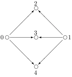
In this section we discuss an important class of toric hyperk¨ahler manifolds, namely, Nakajima’s quiver varieties in the special case when the dimension vector has all coordinates equal to one. Let Q= (V, E) be a directed graph (a
quiver) withd+ 1 vertices V ={v0, v1, . . . , vd} andnedges{eij : (i, j)∈E}.
We consider the group of allZ-linear combinations ofV whose coefficients sum to zero. We fix the basis{v0−v1, . . . , v0−vd} for this group, which is hence identified withZd. We also identifyZnwith the group ofZ-linear combinations
P
ijλijeij of the set of edges E. The boundary map of the quiver Q is the
following homomorphism of abelian groups
A : Zn →Zd, eij 7→ vi−vj. (40)
Throughout this section we assume that the underlying graph ofQis connected. This ensures thatAis an epimorphism. The kernel ofAconsists of allZ-linear combinations of E which represent cycles in Q. We fix an n×(n−d)-matrix B whose columns form a basis for the cycle lattice ker(A). Thus we are in the situation of (1). The following result is well-known:
Lemma 8.1 The matrix A representing the boundary map of a quiver Q is unimodular.
Every edge eij of Q determines one coordinate function zij on Cn and two
coordinate functions zij, wij onHn. The action of the d-torus on Cn and Hn
given by the matrixAequals
zij 7→tit−j1·zij, wij 7→t−i1tj·wij. (41)
We are interested in the various quotients of Cn andHn by this action. Since
the matrixArepresents the quiverQ, we writeX(Q, θ) instead ofX(A, θ), we writeX(Q±, θ) instead ofX(A±, θ), and we write Y(Q, θ) instead of Y(A, θ).
From Corollary 2.9 and Lemma 8.1, we conclude that all of these quotients are manifolds when the parameter vectorθis generic:
Proposition 8.2 Let θ be a generic vector in the latticeZd. Then X(Q, θ) is a smooth projective toric variety of dimension n−d, X(Q±, θ) is a non-compact smooth toric variety of dimension 2n−d, and Y(Q, θ) is a smooth toric hyperk¨ahler variety of dimension2(n−d).
common core of Y(Q, θ) and X(Q±, θ). These manifolds and their core have
the same integral cohomology ring, to be described in terms of quiver data in Theorem 8.3.
Fix a vector θ ∈ Zd and a subset τ ⊆ E which forms a spanning tree in Q.
Then there exists a unique linear combination with integer coefficients λτ ij
ij is non-zero for all spanning treesτ and
all (i, j)∈τ.
Recall that a cut of the quiver Q is a collection D of edges which traverses a partition (W, V\W) of the vertex set V. We regard D as a signed set by recording the directions of its edges as follows
D− = ©
We now state our main result regarding toric quiver varieties:
Theorem 8.3 Letθ∈Zd be generic. The Lawrence toric varietyX(Q±, θ)is the smooth(2n−d)-dimensional toric variety defined by the fan whose2nrays are the columns of Λ(B) =
µI I 0 BT
¶
and whose maximal cones are indexed
by the sets σ(τ, θ), whereτ runs over all spanning trees ofQ. The toric quiver variety Y(Q, θ) is the 2(n−d)-dimensional submanifold of X(Q±, θ) defined by the equations P
(i,j)∈D+zijwij =P(i,j)∈D−zijwij where D runs over all
cuts ofQ. The common cohomology ring of these manifolds is the quotient of
Z[∂ij : (i, j)∈E] modulo the ideal generated by the linear forms in ∂·B and the monomials Q
(i,j)∈D∂ij whereD runs over all cuts ofQ.
A few comments are in place: the variables ∂ij, (i, j)∈E, are the coordinates of
the row vector∂, so the entries of∂·B are a cycle basis forQ. The equations which cut out the toric quiver variety Y(Q, θ) lie in the Cox homogeneous coordinate ring of the Lawrence toric manifold X(Q±, θ). A more compact