Basic NEC
with Broadcast
Basic NEC
with Broadcast
Applications
J.L. Smith, PE
AMSTERDAM • BOSTON • HEIDELBERG • LONDON NEW YORK • OXFORD PARIS • SAN DIEGO • SAN FRANCISCO • SINGAPORE • SYDNEY • TOKYO
Marketing Manager: Christine Degon Veroulis Design Direction: Joanne Blank
Cover Design: Gary Ragaglia Cover Images © J.L. Smith Text Printer: Sheridan Books Cover Printer: Phoenix Color Corp.
Focal Press is an imprint of Elsevier
30 Corporate Drive, Suite 400, Burlington, MA 01803, USA Linacre House, Jordan Hill, Oxford OX2 8DP, UK
Copyright © 2008, Elsevier Inc. All rights reserved.
No part of this publication may be reproduced, stored in a retrieval system, or transmitted in any form or by any means, electronic, mechanical, photocopying, recording, or otherwise, without the prior written permission of the publisher.
Permissions may be sought directly from Elsevier’s Science & Technology Rights Department in Oxford, UK: phone: (⫹44) 1865 843830, fax: (⫹44) 1865 853333, E-mail: [email protected].
You may also complete your request on-line via the Elsevier homepage (http://elsevier.com), by selecting “Support & Contact” then “Copyright and Permission” and then “Obtaining Permissions.”
Library of Congress Cataloging-in-Publication Data
Smith, J.L.
Basic NEC with broadcast applications / J.L. Smith. p. cm.
Includes index.
ISBN 978-0-240-81073-7 (alk. paper)
1. Antenna arrays. 2. Radio—Transmitters and transmission. 3. Transmitters and transmission. I. Title.
TK7871.6.S566 2008
621.384’135—dc22 2008004493
British Library Cataloguing-in-Publication Data
A catalogue record for this book is available from the British Library.
For information on all Focal Press publications visit our website at www.books.elsevier.com
08 09 10 11 12 5 4 3 2 1
To my lovely wife, Marguerite,
who has been in my corner for 63 years.
She assures me that I’m the Champ,
she tells me that I’m winning,
and she pushes me back into the ring
Foreword xiii
Preface xv
Acknowledgments xix
About the Author xxi
CHAPTER 1 The Array Adjustment Process ...1
1.1 The Nature of NEC-2 ...1
1.2 The Directional Antenna Adjusting Process ...1
1.3 Local and Global Minima ...2
1.4 The Role of NEC-2 ...4
1.5 Analysis Overview ...5
1.6 Additional NEC-2 Benefi ts ...6
1.7 Software Requirements ...7
CHAPTER 2 NEC-2 Fundamentals ...9
2.1 Scope ...9
2.2 The NEC-2 Engine ...9
2.3 NEC-2 Operation ...11
2.4 Creating the Input File ...11
2.4.1 Naming the Files ...11
2.4.2 Data Commands ...12
2.4.3 Data Command Types ...13
2.4.4 An Input File Illustration ...13
2.5 Reading the Output File ...17
2.5.1 The Header ...18
2.5.2 Structure Specifi cations ...18
2.5.3 Segmentation Data ...18
2.5.4 Data Commands, Frequency, Loading, and Environment Data ...21
2.5.5 Antenna Input Parameters ...22
2.5.6 Currents and Locations ...22
2.5.7 Current Moments ...23
2.5.8 Power Budget ...24
2.5.9 Radiation Pattern ...24
2.6 Exercises ...26
CHAPTER 3 Modeling the Radiator ...27
3.1 Modeling Guidelines ...27
3.2 Guideline Summary ...29
Contents
3.2.1 Modeling the Radiator ...29
3.2.2 Modeling the Voltage Source ...29
3.3 Tower Confi gurations ...30
3.3.1 Single-Wire Confi guration ...31
3.3.2 Four-Wire Confi guration ...31
3.3.3 Two-Wire Confi guration ...32
3.3.4 Lattice Confi guration ...32
3.4 Viewing Tower Confi guration ...38
3.5 Exercises ...39
CHAPTER 4 Array Geometry ...41
4.1 The Coordinate System ...41
4.2 Array Geometry: An Example ...44
4.3 The Array Input File ...46
4.4 Exercises ...50
CHAPTER 5 Loads, Networks, and Transmission Lines ...51
5.1 Modeling Impedance Loads ...51
5.2 Modeling Nonradiating Networks ...53
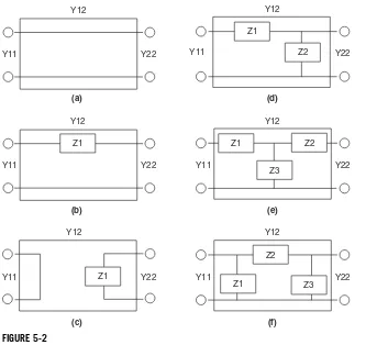
5.2.1 Typical Networks ...54
5.2.2 Typical Network Applications ...55
5.2.3 General Guidelines for Networks ...57
5.3 Modeling Transmission Lines ...57
5.4 Network Output File Listing ...59
5.4.1 Network Descriptions ...59
5.4.2 Source and Load Impedance to the Networks ...60
5.4.3 Network Input Parameters ...61
5.5 Exercises ...61
CHAPTER 6 Calculating Base Drive Voltages ...63
6.1 Base Drive Voltages ...63
6.2 Direct and Induced Currents ...63
6.3 Current Moments ...66
6.4 Development Concept ...67
6.4.1 Unity Drive ...68
6.4.2 Normalized Drive ...69
6.4.3 Full Power Drive ...71
6.4.4 Shunt Reactance and Networks ...71
6.5 Example: A Three-Tower Array ...72
6.5.1 Create a Unity Drive File ...72
ix
Contents
6.5.3 Solve for the Normalized Drive Voltages ...77
6.5.4 Determine the Full Power Drive Voltages ...78
6.6 Exercises ...79
CHAPTER 7 Using Data from the Output File ...81
7.1 Overview ...81
7.2 Verify the Field Ratios ...82
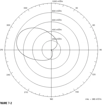
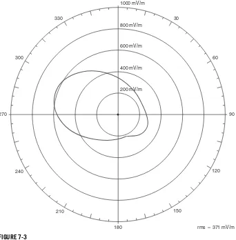
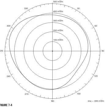
7.3 Plot Far-Field Radiation Pattern ...83
7.4 Detuning Unused Towers ...84
7.4.1 Detuning by Base Loading ...85
7.4.2 Detuning by Skirting ...89
7.5 Antenna Monitor Readings ...94
7.5.1 Optimum Height for Sample Loops ...95
7.5.2 Arbitrary Height for Sample Loops ...96
7.5.3 Base Current Samples ...97
7.5.4 Base Voltage Samples...99
7.6 Drive Point Impedance ...100
7.6.1 Drive Point Impedance When Using a Network ...100
7.7 Exercises ...102
CHAPTER 8 Model by Measurement ...105
8.1 Objective ...105
8.2 Adjusting the Model ...107
8.2.1 Number of Segments ...108
8.2.2 Tower Diameter ...111
8.2.3 Segment and Radius Taper ...114
8.2.4 Base Capacity ...116
8.2.5 Drive Segment Radius ...118
8.3 Exercise...120
CHAPTER 9 Top-Loaded and Skirted Towers ...121
9.1 General Considerations ...121
9.2 Top Loading ...122
9.2.1 Estimating the Size of the Top Hat ...122
9.2.2 Determining the Degree of Top Loading ...123
9.3 Skirted Towers ...126
9.4 Folded Monopole ...129
CHAPTER 10 System Bandwidth Analysis ...133
10.1 Introduction ...133
10.2 System Defi nition ...133
10.2.1 Tower Models ...134
10.2.2 Tower Base Drive Voltages ...136
10.3 Bandwidth Analysis ...137
10.3.1 Source Impedance of the Drive Voltage ...137
10.3.2 Intermediate Data ...140
10.3.3 Total System Bandwidth Data ...146
10.4 Bandwidth Conclusions ...148
CHAPTER 11 Case Studies ...149
11.1 Comparative Data ...149
11.2 Case Study 1: Three-Tower Array ...149
11.2.1 Array Description: Three-Tower Array ...149
11.2.2 Self-Impedance: Three-Tower Array ...149
11.2.3 Antenna Monitor Reading: Three-Tower Array ...151
11.2.4 Array Data: Three-Tower Array ...152
11.2.5 Discussion: Three-Tower Array ...153
11.2.6 NEC-2 Input File: Three-Tower Array ...153
11.3 Case Study 2: Six-Tower Array, Day Pattern ...154
11.3.1 Array Description: Six-Tower Array, Day Pattern...154
11.3.2 Self-impedance: Six-Tower Array, Day Pattern ...154
11.3.3 Antenna Monitor Reading: Six-Tower Array, Day Pattern ...155
11.3.4 Array Data: Six-Tower Array, Day Pattern ...156
11.3.5 Discussion: Six-Tower Array, Day Pattern ...157
11.3.6 NEC-2 Input File ...158
11.4 Case Study 3: Six-Tower Array, Night Pattern ...160
11.4.1 Array Description: Six-Tower Array, Night Pattern ...160
11.4.2 Self-Impedance: Six-Tower Array, Night Pattern ...160
11.4.3 Antenna Monitor Readings: Six-Tower Array, Night Pattern ...160
11.4.4 Array Data: Six-Tower Array, Night Pattern ...161
11.4.5 Discussion: Six-Tower Array, Night Pattern ...161
11.4.6 NEC-2 Input File: Six-Tower Array, Night Pattern ...165
11.5 Case Study 4: Tall-Tower Array ...166
11.5.1 Array Description: Tall Towers ...166
11.5.2 Self-Impedance: Tall Towers ...166
11.5.3 Antenna Monitor Reading: Tall Towers ...167
xi
Contents
11.5.5 Discussion: Tall Towers ...169
11.5.6 NEC-2 Input File: Tall Towers ...169
CHAPTER 12 Supplemental Topics ...171
12.1 Introduction ...171
12.2 Parallel Feeds: Network Combiners ...171
12.3 New Structures: The NX Command ...173
12.4 Numerical Green’s Function ...175
12.5 Ground Screens...177
12.5.1 The GN Command ...177
12.5.2 The GR Command...178
12.6 Finite Ground ...181
12.6.1 Refl ection Coeffi cient Approximation ...182
12.6.2 Sommerfeld/Norton Analysis ...182
APPENDIX A NEC-2 Input File Statements ...185
1.0 Comment Commands (CM, CE) ...187
2.0 Structure Geometry Commands ...189
3.0 Program Control Commands ...211
APPENDIX B Error Messages ...251
APPENDIX C Software ...259
1.1 Introduction ...259
1.2 Disk Content ...259
1.3 Essential Software ...260
2.1 Software Installation ...260
3.1 User Manual ...262
3.1.1 bnec.exe ...262
3.2 NVCOMP.EXE ...263
3.3 NecDrv2.EXE ...265
3.4 NECMOM.EXE ...266
3.5 WJGRAPS.EXE ...266
4.1 Software Support ...267
The development of computer programs for modeling antennas began in the 1960s when main-frame computers were making advancements. Modeling codes that could run on desktop computers made their appearance in the early 1980s. The design of directional antenna arrays for medium-frequency (MF) broadcasting stations has a much longer history, however, reaching back to the mid-1930s when computations were done using a slide rule.
In the early years, methods involving approximations (such as the assumption of sinusoidal current distributions on the radiators) were developed and broadcasters have used them with reasonable success up to the present day. For the most part, however, to do that work the broadcaster’s use of the computer has been relegated primarily to arithmetical operations rather than to actual modeling of the antenna. The success of simple design methods, and the fact that the general-purpose modeling codes and broadcast antenna engineers sometimes seem to “speak a different language,” may account for the somewhat slow adoption of computer modeling by the broadcast community.
J.L. Smith has extensive experience in directional antenna design, which began long before the development of computer modeling. In
Basic NEC with Broadcast Applications, he describes methods he has
developed to use the public domain NEC-2 modeling code to design and tune MF directional antenna arrays. Some of the methods parallel the techniques developed by the navy’s antenna designers by starting with simplifi ed models and sometimes adjusting the models to match measurements. By using these methods, model parameters can be var-ied or features can be added to study effects.
In teaching courses on antenna modeling, we have found that new users often start by trying to model with too much detail. As a result, they run into problems with code limitations and eventually produce a large model that takes a long time to run and makes it diffi cult to try variations. Smith shows how to start with simple models, how to allow for code limitations and still get the important information. He illustrates
Foreword
the effectiveness of his methods by eventually comparing model results to measurements.
This book should be useful for both the beginning student and the working broadcast engineer. Beyond learning the methods described, you will be encouraged to see that it is possible for an ordinary user to get valuable results from the free public domain NEC-2 computer code.
The Numerical Electromagnetics Code version 2 (NEC-2) is a public domain computer program that eliminates most of the shortcomings inherent in the conventional design methods for medium-frequency (MF) broadcast directional antennas. It is most useful for the increas-ingly complex arrays, and it yields parameter settings that greatly aid the initial adjustment of a new array.
NEC-2 was developed at Lawrence Livermore National Laboratories by G. J. Burke and A. J. Poggio in 1981 as a general-purpose tool for the design and analysis of antennas in general. For the most part, its pub-lished applications deal only with antennas that have a single drive source such as those found on dipoles, yagis, rhombics, and so on. Broadcast applications, on the other hand, use multiple sources to indi-vidually drive the separate elements of a multi-element array, with each source having a unique magnitude and phase so as to create a particu-lar radiation pattern.
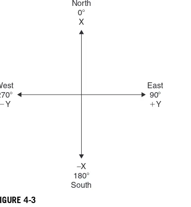
NEC-2 is not necessarily user-friendly to the broadcaster. From the very beginning, it gives the broadcaster a swift kick in the shin when it calls for defi ned source voltages as the inputs to initiate a given antenna analysis, whereas broadcasters have conventionally started their design with a given set of fi eld ratios. Then among other complications, NEC-2 uses the coordinate system common to mathematics, whereas broad-casters have traditionally used the geographical coordinate system. Then NEC-2 deals with peak values, not RMS, as does the broadcaster.
Thus, while NEC-2 is indeed a magnifi cent tool, it is not at all directed to broadcast use. As a result, when NEC-2 fi rst made its appear-ance, it was not immediately accepted by the broadcast community and only a few broadcast engineers even attempted to use it.
In time, however, broadcast engineers with various levels of exper-tise studied the use of NEC-2 and each developed their own postpro-cessing software to read data from the standard output fi le and to use that data to perform the various tasks necessary for broadcast work. Such studies have been carried on rather independently, and some-what privately, however, and some engineers even consider their work
Preface
proprietary. Unfortunately, little of the work has been published to enjoy peer review or to serve as tutorials for those seeking entry into the profession.
In recent years, some engineers have written software to make the moment method programs more user-friendly to the broadcaster, and some of the more developed efforts have been packaged as commer-cial products for sale to the broadcast community. The consensus is, however, that the commercial products all use the same basic moment method engine and that they differ mainly in the user interface with, perhaps, some special features added.
Because there has been such a diversity in the development of the procedures for applying NEC-2 calculations to broadcast arrays, there may be multiple approaches to accomplish a given analysis, and each approach possesses merit. Therefore, as you study NEC-2 from this book and other sources, you might fi nd additional and even contradicting methods of analysis; in that case, I encourage you to weigh the merits of each and to exercise your judgment as to the best use of available methods.
At the present time, there is no modern and comprehensive tuto-rial available to a person desiring to enter the fi eld of MF directional antenna design, and the few remaining people who are knowledge-able of the science are becoming older and, unfortunately, fewer. This regrettable circumstance occurs at a time when we are on the brink of a resurgence of need as new forms of modulation make their way into the MF band. Digital modulation methods make it necessary to renew our interest in directional antenna systems as we study bandwidth requirements and learn new implementation schemes to accommodate the more sophisticated application. At the same time, 5000 existing directional antenna systems continue to demand maintenance, and the need for replacement grows as they come to their life’s end at the rate of approximately 100 per year.
Basic NEC with Broadcast Applications was written to show how
xvii
the professional user of the many details encountered while using NEC-2 to analyze and design modern MF directional antenna arrays.
Finally, a somewhat lofty goal is that others more skilled in the science than I will see this book as an incentive to make their own contributions to publicly documenting the use of NEC for broadcast applications.
Someone once said, “We see the future by standing upon the shoulders of those who have gone before us.” While I don’t mean to imply that the following persons have preceded me in time (for I’m much too old for that), I do want to acknowledge that they have preceded me in knowledge and that they have given of that knowledge generously to make this book possible.
My sincere appreciation goes to the many people who have contrib-uted to this book, but I am especially indebted to:
■ Gerald J. (Jerry) Burke, of Lawrence Livermore National Laboratory
and cocreator of NEC-2, who gave so generously of his time to review this manuscript and to make many valuable suggestions.
■ Jack Sellmeyer, Sellmeyer Engineering, McKinney, TX, and former
coworker at Collins Radio Company, whose contributions and patience through the years have provided the practical experi-ence necessary to bring realism to theory.
■ Paul Carlier, FanField, Ltd., UK, for his contribution to, and review
of, that portion of the manuscript pertaining to measured data.
And for years of discussions and the sharing of practical experience, I express my sincere appreciation to my long-time friend, Paul Cram, Broadcast Technical Services, Mansfi eld, GA, who started working with directional antennas when the concept fi rst appeared in 1935. Now in his nineties, Paul is still in the profession and aggressively applying NEC-2 to broadcast directional antennas.
Acknowledgments
J.L. Smith received a B.S. degree in physics from the University of Houston in 1956 and an M.S. degree in engineering from Southern Methodist University in 1959. He began his career in broadcasting at KTRH in Houston in 1946. In 1956, he joined Collins Radio Company where he held the usual positions in research and development cul-minating in head of the Department of Research and Development. He served as the manager of Broadcast Systems Engineering at Collins Radio Company during the 1960s. While there he directed the develop-ment of a complete catalog of new broadcast products.
Mr. Smith has been active in FCC matters, having fi led the fi rst petition advocating automatic unattended operation of FM broad-cast transmitters. He participated in the coordination of international broadcasting through his service on CCIR Study Group 10 and has participated in various national and international symposia. J.L. Smith has authored approximately 50 technical papers and has published two other books—Basic Mathematics with Electronics Applications (Macmillan, 1972) and Intermodulation Prediction and Control (Interference Control Technologies, 1993).
He is now retired in Covington, Louisiana, where he devotes much of his time to analytical research pertaining to AM directional antennas.
About the Author
1
CHAPTER
1.1
The Nature of NEC-2
It is important to recognize that the Numerical Electromagnetics Code (NEC) is no magic tool—it does some things very well but it cannot do other things. In spite of this, it is a valuable tool that makes a signifi cant contribution to easing the design and adjustment of medium-frequency (MF) broadcast directional antennas.
The user of NEC-2 should have realistic expectations, and recog-nize from the outset, that the results of a NEC-2 analysis are, at best, an approximation, and they are not necessarily exact answers. Fortunately, however, the results of a NEC-2 analysis need not be precise to be benefi cial.
1.2
The Directional Antenna Adjusting Process
The process of physically adjusting the network components of an array to achieve a desired pattern is very similar to that of mathemati-cally synthesizing a radiation pattern using computerized optimiz-ing methods. Both processes start with a given pattern, compare it to a target, determine an error, and then make parameter adjustments in an attempt to reduce the error. In the physical adjustment process, the pattern error is a matter of human opinion; in the case of computerized pattern synthesis, the error is defi ned mathematically.
The Array Adjustment
The mathematical synthesis process and the physical adjustment process possess the same signifi cant limitation in that neither can know when the minimum error has actually been reached. Therefore, in both cases the usual practice is to test a potential error minimum by changing a parameter value and noting the effect on the error. If the error increases, then the parameter is returned to its original value and another parameter value is changed. If all the parameter values are changed in turn and none reduces the error, then it is often assumed that the error is at a minimum.
The task does not end there, however. The error may indeed be at a minimum, but it may not be at the absolute minimum. There may be another set of parameters that will create an even smaller error. That concept can be better understood by considering the following analogy.
1.3
Local and Global Minima
The pattern error can be envisioned as an N⫹ 1 dimension surface
where N is the number of variables.
Figure 1-1 shows a three-dimensional error surface of two variables, arbitrarily called Field Ratio and Phase for example purposes. Point S in Figure 1-1 is taken as an arbitrary starting point from which we
Field ratio
Error
Phase
M' M S
S'
FIGURE 1-1
3
will make a search in an effort to fi nd point M, which is the point on the surface representing the values of Field Ratio and Phase where the error is least.
The object is to change the values of Field Ratio and Phase so as to move from point S to point M. That is not necessarily a simple task, especially if there are more than two variables. One must know not only which variable to change, but also the direction of the change and how much change is required. Ultimately, however, after a number of changes, a point will be reached where an additional change of either variable will cause the error to increase. It might then be concluded that point M has been reached.
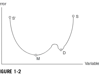
Only the simplest arrays have smooth error surfaces, as shown in Figure 1-1. The more complex arrays are pock-marked with variations that may be viewed as downward-pointing dimples in the surface. These dimples press the surface down for a range then allow it to rise again. Figure 1-2 shows such a dimple but, for the sake of simplicity, only a one-variable error curve is shown.
Again point S is the starting point in the search for the minimum at point M. Notice, however, that to follow the curve from point S to point M, one must go through point D. While point D suggests that it is the minimum (i.e., at point D the error increases if the variable is varied in either direction), the reduced error at point D is larger than the error at point M. Point M is unique; that is, there can be only one point of least error, so point M is called the global minimum. Point D, on the other hand, is not unique because there can be several points of this type. Therefore, points such as D are called local minima. When adjusting a
Variable Error
S
D M
S'
FIGURE 1-2
Single-variable error curve containing a local minimum.
directional array to a target pattern, then in essence, one must journey along the error surface attempting to reach the global minimum. If the error surface does not continuously increase or decrease but instead has a number of dimples, then one may well fall into a dimple and be in a local minimum. Unfortunately, it is not possible to know that it is a local minimum, nor is there a way to determine that it is a local minimum.
Usually, if the error in a minimum is tolerable, then the adjustment process will be stopped, notwithstanding whether the minimum is local or global. This happens more often than not when physically adjust-ing a complex array.
If the error in the local minimum is intolerable, however, then a new starting point must be chosen and a new adjustment process started from there, hoping to bypass any local minima. For example, if the starting point in Figure 1-2 is changed from point S to point S⬘, it is obvious that
the journey along the curve to point M will occur without complications.
1.4
The Role of NEC-2
The idea to convey here is that if the array is simple, then the error surface is likely to be smooth and the probability of reaching the global minimum is high. If the array is complex, however, then the error sur-face may contain several local minima and the probability of reaching the target without falling into a local minimum is practically zero; so the search process must be repeated over and over . . . unless the start-ing point is initially chosen to be very near the global minimum. This is where NEC-2 makes its contribution.
5
1.5
Analysis Overview
Unless the reader has previous knowledge of the use of NEC-2, it is not likely that the following steps for NEC-2 analysis will be self-explanatory. Nevertheless, the procedure is presented here as an overview to let the reader know what to expect and what the explanations that follow are seeking to accomplish. So if questions remain after fi nishing this sec-tion, be patient; more detail will be revealed in later chapters.
When using the public domain software furnished on the CD included with this book, it is necessary to make three separate NEC-2 runs to arrive at the NEC-2 output fi le that yields the fi nal analysis. Fortunately, this is not diffi cult; nor is it excessively time consuming and the results are just as valuable as those obtained with any commercial software that might have a more user-friendly interface. The NEC-2 computations are made using a slightly modifi ed version of the public domain NEC-2 pro-gram called bnec.exe (included on the CD with this book).
The sequence leading to a NEC-2 analysis proceeds according to the following steps.
1. Create a NEC-2 unity drive input fi le that excites each tower individually with 1.0 ⫹ j0 volts while the companion towers are
grounded. Using that unity drive fi le as the input fi le, run bnec.exe. 2. Using the NEC-2 output fi le created by step 1, run the NecDrv.exe
computer program included on the associated disk to determine the normalized base drive voltages corresponding to the target fi eld ratios.
3. Create a NEC-2 normalized drive input fi le that excites the tow-ers simultaneously with the normalized base drive voltages deter-mined in step 2. Run bnec.exe with that normalized drive fi le as the input fi le.
4. Using the NEC-2 output fi le created by step 3, run the NecMom.exe program included on the associated disk to confi rm that the nor-malized base drive voltages do, in fact, create the target fi eld ratios. 5. Scale the normalized base drive voltages determined in step 2 to
the full power level (described in Chapter 6 of this book) to gen-erate the desired power output.
6. Create a NEC-2 full-power drive input fi le that excites the tow-ers simultaneously with the full-power base drive voltages deter-mined in step 5. Using that full-power drive fi le as the input fi le, run bnec.exe.
7. The NEC-2 output fi le created by step 6 contains the fi nal data for analysis.
Later chapters in this book will show how to interpret the output fi le to learn the peak values of voltages and current at signifi cant points in the system plus how to read the operating drive point impedance of each tower. Armed with this information, the engineer may calculate the antenna-matching networks and set the individual network compo-nent values to a reasonable starting value in preparation for the initial turn-on of the array.
Perhaps the most benefi cial result of a NEC-2 analysis is the current distribution listing for each tower of the array. From these current dis-tribution listings, the designer can determine at what height to position the antenna monitor sampling loops such that the antenna monitor will give indications that closely correspond to the associated far-fi eld ratios. He can also determine the base voltage ratios corresponding to the target fi eld ratios if his antenna monitor samples those voltages.
If the sample loops are not positioned at the optimum height, or if current transformers are used to sample the tower current, then the NEC-2 current distribution listing can be used to determine the moni-tor reading that corresponds to the desired far-fi eld ratio.
Thus, with some indication of the radiated far-fi eld ratios at hand during the initial adjustment process, the array networks can be adjusted to very near their fi nal values without the benefi t of distant-fi eld strength measurements and without being plagued by falling into a local minimum.
1.6
Additional NEC-2 Benefi ts
7
First, a NEC-2 analysis allows the engineer to explore physical arrange-ments that are not practical using hardware—the effects of different tower heights, for example. In addition, the engineer is able to examine the impact of unused towers and other structures in the vicinity of the array. He or she is able to study the effects of top loading and tower skirts, as well as shunting reactance at the tower insulator. NEC-2 also gives good indications of power budget, currents, impedances, and so on.
In summary, the results obtained from the NEC-2 analysis may not be exact, but they still provide the engineer with an insight into array performance that minimizes the “cut-and-try” effort so common to array adjustment.
1.7
Software Requirements
Antenna analysis software sells for as much as $2000 or more and many of the commercial computer programs being sold for that purpose use the basic NEC-2 or NEC-4 engine. They differ, for the most part, only in the way they present a convenient or novel user interface.
Therefore, in the interest of economy, this book uses the NEC-2 pub-lic domain software that can be downloaded from the Internet free of charge. The human interface with the public domain software may not be as elegant as some of the purchased products, and the public domain software may not be as user-friendly, but the results are just as useful and just as rewarding, and the time spent in learning to use it is indeed invested wisely.
If, however, the reader already possesses commercial software, then in most cases the commercial software can be used in lieu of the pub-lic domain software. The concepts presented in this book are valid independently of the software used. And while the postprocessing pro-grams furnished on the associated disk may not be compatible with the output format of the commercial software, suffi cient information is furnished in the book to allow one to write simple postprocessing pro-grams that are compatible with the output fi les at hand.
9
CHAPTER
2.1
Scope
As the name implies, this book covers only the basic application of NEC-2 to the design and analysis of MF directional antennas. The essen-tials are described in suffi cient detail to teach the useful design and analysis of medium-frequency (MF) broadcast antenna arrays, but some refi nements of NEC-2 are not specifi cally described in this text or they are given only cursory mention. Some of these refi nements include the use of symmetry and refl ection to simplify the input fi le, wire arcs, dimension scaling, and multiple structures. Only a cursory explanation of the use of Numerical Green’s Function and the Sommerfeld/Norton fi nite-ground method is given in the last chapter so more study will be needed to fully exploit those topics.
In addition, NEC-2 has some capabilities that are not usually associ-ated directly with broadcasting; therefore, those topics are not included in this text. These include the ability to model helix and cylindrical structures, surface patches, and circular and elliptical polarization.
However, to augment the material in the text, Appendix A includes the complete catalog of NEC2 commands. They are described in suffi -cient detail in the appendix to permit the reader to individually extend study to any capability of NEC-2.
2.2
The NEC-2 Engine
The Numerical Electromagnetics Code was written in 1977 by G. J. Burke and A. J. Poggio at Lawrence Livermore National Laboratory under
NEC-2 Fundamentals
contract to the U.S. Navy. The code was originally known as the Numerical Electromagnetics Code (NEC). As the code was improved over time, it was renamed NEC-2 in 1980, NEC-3 in 1983, and ulti-mately NEC-4 in 1990. NEC-2 has been declared public domain, NEC-3 no longer exists, and the distribution of NEC-4 is controlled by licens-ing through the Industrial Partnership and Commercialization Offi ce at Lawrence Livermore National Laboratory.
The NEC-4 source code is an extensive revision of the NEC-2 code that makes more use of the Fortran 77 constructs and is more modu-lar and easier to understand and maintain. Additional features and capa-bility were added in the revision process. For example, NEC-2 models wire structures both in free space and over a ground plane. The ground plane may be either perfectly conducting or have fi nite ground char-acteristics. NEC-4 possesses the same abilities as NEC-2 in this regard plus it is able to model wire structures buried in the ground or passing through the air/ground interface.
NEC-4 also carries revisions of the NEC-2 code that reduce the loss of precision when modeling tightly coupled wires and electrically small structures. In addition, NEC-4 has been changed to be more accurate than NEC-2 when treating models containing stepped-radius wires or junctions of wires of differing radius. NEC-4 can also accommodate the effects of insulated wires, whereas NEC-2 has no such provision.
Thus, while NEC-4 is, indeed, considered the most accurate, NEC-2 is quite adequate for most broadcast applications. Therefore, because NEC-2 is in the public domain and available at no charge, it was selected to be the code used in this book.
Both the executable and source code for NEC-2 are widely distrib-uted on the Internet and the code has been liberally modifi ed by vari-ous users. The NEC-2 computer program used in this book is a modifi ed version of NEC2dxs.zip. At the time of this writing, NEC2dxs.zip can be downloaded free of charge from the Internet: http://www.si-list.
net/swindex.html.
11
been modifi ed slightly to make the GM command input format more useful to the broadcaster and to dimension the arrays to accommo-date a 120 wire ground screen. It has also been changed to protect the input fi le from accidental erasure. Please be aware that the GM command (described in Chapter 3) has been modifi ed. It is compat-ible with bnec.exe, but the modifi ed version is not compatcompat-ible with the usual NEC2dxs programs. The GM command used here is, however, compatible with the NEC-4 fi le format. Therefore, the input fi les gener-ated during the study of this book are, for the most part, usable with both bnec.exe and NEC-4.
2.3
NEC-2 Operation
In perhaps an oversimplifi ed explanation, the antenna to be analyzed is modeled by a series of wires and voltage sources as described to NEC-2 in an input fi le furnished by the user. When run, NEC-2 divides each wire into the number of segments specifi ed by the user. It then calcu-lates the current on each segment and fi nally sums the effects of all segments to get a fi nal result. NEC-2 stores its output in a fi le that it places in the computer’s currently active folder. The user must recall the output fi le to read, print, or otherwise use it.
2.4
Creating the Input File
To use NEC-2, the user must generate an input fi le that describes the antenna geometry and operating parameters in a defi ned format. This is done using any convenient text editor and saving the fi le in text form. When NEC-2 is run, it issues a call for the path and name of the input fi le plus the name that the user wishes to assign to the output fi le. There are no other communications with the user while NEC-2 runs.
2.4.1 Naming the Files
During the course of conducting a directional array analysis, it is neces-sary to make several NEC-2 runs and to generate several NEC-2 input
and output fi les. To conveniently keep track of the various fi les, a nam-ing convention is recommended. The convention used in this book is defi ned as we go along and the reader is encouraged to follow that con-vention to avoid confusion.
In that regard, it is suffi cient to say at this time that all fi les may be named with the call letters of the station using the antenna array. For some discussions in this book, CALL will represent a generic station call being used for illustration purposes. All input fi les will carry the exten-sion .NEC. Thus, the input fi le will be named CALL.NEC. The output fi le generated by NEC-2 when CALL.NEC is the input fi le can be named anything but it is highly recommended that it be named CALL.OUT.
2.4.2 Data Commands
The original NEC-2 computer program used punched cards to input the data that describes an antenna and to request computation of antenna characteristics. But, as mentioned earlier, modern NEC-2 now uses an input text fi le with the format of the data within that fi le being similar to that of the punched card set. Each line in the input fi le is a separate command and each command carries the data that initially appeared on a single punched card. Instead of the data being written into positional fi elds, however, modern NEC-2 fi les use data fi elds delimited by com-mas or spaces. Because of the similarity to a punched card set, and of course the inertia of habit, each data statement command in the input fi le is sometimes referred to as a “card.” However, in an attempt to be more descriptive, this book follows the precedent set by the documen-tation of NEC-4 and uses the word “command” rather than the word “card” when referring to the statements in the input fi le.
A typical data command is:
RP 0, 1, 361, 1001, 90., 0., 0., 1., 1609., 0.
The commands in an input fi le must be written in ASCII text and they must begin in column 1 of line 1. Each successive command must then begin in column 1. Do not indent the commands or use spaces at the beginning of the commands and do not use blank lines.
13
two-letter command codes in the NEC-2 vocabulary and all of them are given in Appendix A. However, only about 20 of these codes are nor-mally used in broadcast calculations. The simple example that follows later uses only 9 of the command codes and those are probably the most common command codes used by broadcasters.
All commands having numeric data are written in a similar format, with fi elds for integer numbers fi rst, followed by fi elds for real num-bers. Integer numbers are written with no decimal point. Real numbers are written as a string of digits and may contain a decimal point. Real numbers may also be written as a string of digits containing a deci-mal point followed by an exponent of 10 in the form 1.234E⫾6. This is interpreted as multiplying the number 1.234 by 10⫾6.
2.4.3 Data Command Types
The input fi le for a single NEC-2 run must contain at least one of each of the three types of command.
1. The input fi le must begin with one or more comment commands that can contain any type of information but they usually provide a description of the NEC-2 run. This information is printed at the start of the output fi le as a label.
2. The comments are followed by geometry commands, which describe the antenna system. The geometry commands have two fi elds for integer numbers followed by real-number fi elds as necessary.
3. Finally, a number of program control commands specify electrical parameters such as frequency, loading, and excitation. Commands of this type also request the execution of the .NEC fi le. The pro-gram control commands have four integer fi elds followed by real-number fi elds.
2.4.4 An Input File Illustration
The following illustration is included here to stimulate the reader’s interest before we embark upon a series of long explanations. A single
tower is used in this example because it is the simplest representation. Of course, a broadcast array will have multiple towers. The object of this one-tower calculation might be to determine the driving point impedance of the tower, although enough data is included in the out-put fi le to enable one to plot the current distribution on the tower and to view the antenna radiation pattern.
Remember that the data commands in an input fi le must begin in column 1 of line 1. Each successive command must then begin in col-umn 1. Do not indent the commands or use spaces at the beginning of the commands and do not use blank lines.
The example input fi le listed here contains three comment com-mands (CM, CM, CE), two geometry comcom-mands (GW, GE), and fi ve pro-gram control commands (GN, FR, EX, RP, EN). A full explanation of all the input commands is given in Appendix A. As each command code is addressed in the paragraphs that follow, the reader is encouraged to read the full description of that command code as it appears in Appendix A.
The commands in Listing 2-1 make up the sample input fi le.
Comment Commands
Every input fi le must contain at least one comment command and if there is only one comment command, it must be the CE command. Any other comment commands must precede the CE command and must be identifi ed as CM commands. In the preceding example. CM and CE are comment commands.
Geometry Commands
Several types of geometry command can be used to describe the wires in an antenna but the GW is the most used for broadcast work. The
Listing 2-1
CM This is a comment line – usually shows the fi le name, CALL.NEC CM The comment lines will be printed in the Output fi le.
CE The last comment line must use the CE designation. GW, 101, 20, 0., 0., 0., 0., 0., 115., 0.5
GE,1 GN,1
FR, 0, 1, 0, 0, 1.5, 0.
EX, 0, 101, 1, 00, 1266.084, 0.
15
GW command describes a straight wire located in an XYZ coordinate system where lengths are measured in meters. For our broadcast work, towers are considered to be wires or to be made up of a group of wires. The simplest description of an antenna tower is a single vertical wire of defi ned radius, as represented in the GW command of Listing 2-1.
The position of each wire must be specifi ed and the number of seg-ments into which the wire is to be divided must also be specifi ed. The position of a wire is defi ned by showing the coordinates of each end, as presented in the XYZ coordinate system. While you must specify the number of segments, it is not necessary to defi ne the position of each segment because NEC-2 does this routinely. While only one wire is used in the simple example above, multiple wires can be used to describe a single tower and, of course, multiple wires are used to describe a multi-tower directional array.
Referring to the GW wire in Listing 2-1, the number 101 is the wire tag number assigned to identify this wire. By broadcast convention, the 100 tag series (101, 102, 103, etc.) is used to identify wires associated with tower 1. The 200 series (201, 202, 203, etc.) identifi es wires asso-ciated with tower 2; the 300 series, tower 3, and so on. Be sure to get into the habit of using this convention because some postprocessing programs take advantage of this convention to identify towers and to determine the number of towers in an array.
In Listing 2-1, the wire tag 101 in the GW command shows that this is wire 1 of tower 1. Next, the digits 20 show that we have elected to divide the wire into 20 segments. The next three fi elds show that the fi rst end of the wire is located at X ⫽ 0 meters, Y ⫽ 0 meters, and
Z⫽ 0 meters (ground level at the origin). The following three fi elds
show that the second end of the wire is located at X ⫽ 0 meters, Y ⫽ 0
meters, Z ⫽ 115 meters. This describes a vertical tower (wire) located
at the origin and 115 meters high. The last fi eld of the GW command shows that the effective radius of the tower is defi ned to be 0.5 meters.
Next is the GE command, which is mandatory and indicates the end of the geometry description. The GE command also signals whether the antenna is in free space or whether it is operating over a ground plane. GE with no following digit, or with the digit 0 following, indicates free space operation, whereas GE with the digit 1 following is used when a ground plane is present. The GE command does not specify the characteristics of the ground plane; it only readies NEC-2 to accept the ground-plane
parameters from a following command. If a ground plane is present, then in addition to the GE command, the GN command must be included to defi ne the characteristics of that ground plane. Please read the full description of the GE command and the GN command in Appendix A.
Program Control Commands
The GN command is a program control command and shows the characteristics of the ground in the immediate vicinity of the antenna. Appendix A explains that the digit 1 following GN shows that the ground plane is perfectly conducting. A zero or 2 following GN indi-cates a fi nitely conducting ground, which must be defi ned in the remaining fi elds of the GN command. The fi nitely conducting ground is used only in calculating radiated fi elds. The NEC-2 calculated value for the self-impedance of the tower will be the same whether using a perfecting conducting ground or a ground with fi nite constants. Please refer to appendix A for more details on the GN command.
The FR command sets the frequency to 1.5 MHz, although it is capa-ble of doing more. See Appendix A for a full description of the use of the FR command.
The fi rst zero on the EX command shows we are exciting the wire with a voltage source. The following two data fi elds showing wire tag 101 and segment 1 place the excitation on wire 1 of tower 1 using seg-ment 1. The excitation is defi ned to be 1266.084 ⫹ j0 volts by the last
two fi elds of the EX command. Notice that the excitation voltage is a complex number expressed by its real and imaginary parts; thus, it has both magnitude and phase.
It is important to say here that modeling voltage sources is a criti-cal step in the analysis of broadcast antennas. NEC-2 offers two mod-els for voltage sources, the applied-fi eld source and the bicone source. The applied-fi eld source (I1 ⫽ 0 on the EX command) is most
appro-priate for broadcast work. See the EX command in Appendix A for a full explanation.
17
included. Again, refer to Appendix A to read the full description of each of these commands.
As an exercise, type the input fi le commands given as Listing 2-1 in Section 2.4.4 into a fi le and save it as a text fi le with the name CALL.NEC. Any convenient text editor may be used—the EDIT command in Windows works fi ne, as does WordPad and Notepad. If WordPad or Notepad is used, be sure to save the work as a text fi le.
2.5
Reading the Output File
To run the CALL.NEC input fi le using bnec.exe, place CALL.NEC and bnec.exe in the same folder, then run bnec.exe. The bnec.exe will ask for the name of the input fi le, which is CALL.NEC. It will then ask for the name that you wish to assign to the output fi le, and an appropriate response is CALL.OUT. When bnec.exe fi nishes its run, it will leave the output fi le (CALL.OUT) in the currently active folder.
If your input fi le contains an error, NEC-2 does not signal that error during the run time. Instead, it records the error in the output fi le and aborts the run if it is a fatal error. Therefore, you must examine the out-put fi le to identify an error. A brief description of the error will appear at the place in the output fi le where the error occurred. More error descriptions are given in general in Appendix B.
The output fi le can be quite long and it contains some lines lon-ger than 100 characters; thus, it is diffi cult to read in a DOS window. The output fi le is most conveniently viewed using WordPad and called by a batch fi le whose location is included in the PATH variable of the AUTOEXEC.BAT fi le. While on this subject, it is recommended that you also include bnec.exe and a viewing program (described in Appendix C) called NVCOMP.EXE in the PATH variable of the AUTOEXEC.BAT fi le. This will make it more convenient for you to make calculations from any folder.
A satisfactory hard copy of the output fi le can be printed in the por-trait orientation by changing the font of the entire fi le to size 6. The font can be changed to size 8 if the fi le is printed in the landscape ori-entation. (Listings and outputs are shown in 8.5 point Trade Gothic font throughout this book.)
Portions of the fi le CALL.OUT are displayed next with commentary. Please refer to your own printout if you have made one.
2.5.1 The Header
The header and comment lines are displayed at the start of the output fi le. See Output 2-1.
2.5.2 Structure Specifi cations
The wire geometry commands are listed under the heading
- STRUCTURE SPECIFICATION -, as shown in Output 2-2.
Only one wire has been used in this example. Had additional wires been used, they would have been shown as additional printed lines in the output fi le and would be numbered under the heading WIRE NO..
For verifi cation purposes, the X1, Y1, and Z1 headings show the coor-dinates of wire end 1. The coorcoor-dinates of wire end 2 are X2, Y2, and Z2 and the wire radius is listed. The number of segments on the wire is shown, as well as the identifying numbers for those segments and the associated wire tag number.
The presence of a ground plane is verifi ed, as is the ground image. A table of multiple-wire junctions listing any junctions at which three or more wires join is shown next, although this example has none. When multiple-wire junctions are present, the number of each segment connecting to the junction are printed, as a positive number if the refer-ence direction of the segment is into the junction or a negative number if the reference direction is out of the junction.
2.5.3 Segmentation Data
Segment data is printed as shown in Output 2-3 (see page 20) under the heading-SEGMENTATION DATA - together with the angles ALPHA and BETA.
19
Within the subheading CONNECTION DATA the numbers under I⫺
and I⫹ indicate the conditions at the fi rst and second ends of
seg-ment number I, respectively. Segseg-ments connected at a junction can be located by tracing connection numbers through the table. After the sign is dropped, the connection number under I⫺ or I⫹ is the number
of the segment connecting to the end of segment I. If the sign of the connection number is positive, the segment reference directions are aligned (end 1 to end 2 or vice versa); if the number is negative, the Output 2-2
STRUCTURE SPECIFICATION
COORDINATES MUST BE INPUT IN
METERS OR BE SCALED TO METERS
BEFORE STRUCTURE INPUT IS ENDED
WIRE NO. OF FIRST LAST TAG
NO. X1 Y1 Z1 X2 Y2 Z2 RADIUS SEG. SEG. SEG. NO. 1 0.00000 0.00000 0.00000 0.00000 0.00000 115.00000 0.50000 20 1 20 101
GROUND PLANE SPECIFIED.
WHERE WIRE ENDS TOUCH GROUND, CURRENT WILL BE INTERPOLATED TO IMAGE IN GROUND PLANE.
TOTAL SEGMENTS USED⫽ 20 NO. SEG. IN A SYMMETRIC CELL⫽ 20 SYMMETRY FLAG⫽ 0
MULTIPLE WIRE JUNCTIONS
-JUNCTION SEGMENTS (- FOR END 1, + FOR END 2) NONE
2.5Reading the Output File
Output 2-1
*********************************************** the ARRAY DESIGN system
NEC-2dxs (mod)
***********************************************
COMMENTS
-This is a comment line - usually shows the fi le name, CALL.nec The comment lines will be printed in the Output fi le
reference directions are opposed (end 1 to end 1 or end 2 to end 2). When more than one segment connects to a segment end, the connec-tion number gives the next connected segment in the sequence of seg-ments, searching cyclically through the list.
At a free end where the segment ends connects to nothing, the con-nection number is equal to zero.
One way of viewing the connection data is to recognize that the middle column is the segment of interest. To its right (I⫹) is the
num-ber of the next segment to which it connects. To its left (I⫺) is the
number of the previous segment to which it is connected.
For example, notice the fi rst entry, it is segment 1. To the right, it con-nects to segment 2. To its left, it concon-nects to itself (segment 1) because the tower in this example is mounted over a perfectly conducting ground plane. Thus, the tower is connected to an image of itself in the ground. Output 2-3
SEGMENTATION DATA
-COORDINATES IN METERS
I+ AND I- INDICATE THE SEGMENTS BEFORE AND AFTER I
SEG. COORDINATES OF SEG. CENTER SEG. ORIENTATION ANGLES WIRE CONNECTION DATA TAG
NO. X Y Z LENGTH ALPHA BETA RADIUS I– I I+ NO.
1 0.00000 0.00000 2.87500 5.75000 90.00000 0.00000 0.50000 1 1 2 101 2 0.00000 0.00000 8.62500 5.75000 90.00000 0.00000 0.50000 1 2 3 101 3 0.00000 0.00000 14.37500 5.75000 90.00000 0.00000 0.50000 2 3 4 101 4 0.00000 0.00000 20.12500 5.75000 90.00000 0.00000 0.50000 3 4 5 101 5 0.00000 0.00000 25.87500 5.75000 90.00000 0.00000 0.50000 4 5 6 101 6 0.00000 0.00000 31.62500 5.75000 90.00000 0.00000 0.50000 5 6 7 101 7 0.00000 0.00000 37.37500 5.75000 90.00000 0.00000 0.50000 6 7 8 101 8 0.00000 0.00000 43.12500 5.75000 90.00000 0.00000 0.50000 7 8 9 101 9 0.00000 0.00000 48.87500 5.75000 90.00000 0.00000 0.50000 8 9 10 101 10 0.00000 0.00000 54.62500 5.75000 90.00000 0.00000 0.50000 9 10 11 101 11 0.00000 0.00000 60.37500 5.75000 90.00000 0.00000 0.50000 10 11 12 101 12 0.00000 0.00000 66.12500 5.75000 90.00000 0.00000 0.50000 11 12 13 101 13 0.00000 0.00000 71.87500 5.75000 90.00000 0.00000 0.50000 12 13 14 101 14 0.00000 0.00000 77.62500 5.75000 90.00000 0.00000 0.50000 13 14 15 101 15 0.00000 0.00000 83.37500 5.75000 90.00000 0.00000 0.50000 14 15 16 101 16 0.00000 0.00000 89.12500 5.75000 90.00000 0.00000 0.50000 15 16 17 101 17 0.00000 0.00000 94.87500 5.75000 90.00000 0.00000 0.50000 16 17 18 101
18 0.00000 0.00000 100.62500 5.75000 90.00000 0.00000 0.50000 17 18 19 101
19 0.00000 0.00000 106.37500 5.75000 90.00000 0.00000 0.50000 18 19 20 101
21
Look now at the last entry in Output 2-3. It is segment 20. To the left of 20 is 19, which shows that the previous segment is 19. To the right is a zero, so segment 20 is open at that end.
Although it is not used very much in broadcast work, the utility of this listing will be more apparent when a more complex structure is displayed.
While the preceding may assist in confi rming the correctness of the antenna geometry, there are several public domain programs available that will graphically display the antenna model. The program NVCOMP. EXE is one of these and is included on the disk associated with this book. Its use is covered in more detail in Appendix C.
2.5.4 Data Commands, Frequency, Loading, and Environment Data
Output 2-4 shows that the program control commands are listed in the output fi le for verifi cation; the frequency and wavelength are stated;
Output 2-4
* DATA CARD NO. 1 GN 1 0 0 0 0.0000E+00 0.0000E+00 0.0000E+00 0.0000E+00 0.0000E+00 0.0000E+00 * DATA CARD NO. 2 FR 0 1 0 0 1.5000E+00 0.0000E+00 0.0000E+00 0.0000E+00 0.0000E+00 0.0000E+00 * DATA CARD NO. 3 EX 0 101 1 0 1.2661E+03 0.0000E+00 0.0000E+00 0.0000E+00 0.0000E+00 0.0000E+00 * DATA CARD NO. 4 RP 0 1 9 1001 9.000E+01 0.0000E+00 0.0000E+00 4.5000E+01 1.6090E+03 0.0000E+00
FREQUENCY
-FREQUENCY= 1.5000E+00 MHZ WAVELENGTH= 1.9987E+02 METERS
APPROXIMATE INTEGRATION EMPLOYED FOR SEGMENTS MORE THAN 1.000 WAVELENGTHS APART
STRUCTURE IMPEDANCE LOADING
THIS STRUCTURE IS NOT LOADED
ANTENNA ENVIRONMENT
PERFECT GROUND
MATRIX TIMING
-FILL= 0.000 SEC., FACTOR= 0.000 SEC.
Output 2-5
ANTENNA INPUT PARAMETERS
-TAG SEG. VOL-TAGE (VOLTS) CURRENT (AMPS) IMPEDANCE (OHMS) ADMITTANCE (MHOS) POWER
NO. NO. REAL IMAG. REAL IMAG. REAL IMAG. REAL IMAG. WATTS
101 1 1.2661E+3 0.00E+0 1.5797E+0 3.6541E+0 1.2620E+2 –2.9193E+2 1.2477E–3 2.8861E–3 1.000E+3
and if any segments had been impedance loaded (as is covered in Chapter 5), the loading will be listed for verifi cation. The ground condi-tions are also shown together with some timing information.
2.5.5 Antenna Input Parameters
The data in Output 2-5 is very important to the broadcaster because it shows the drive point impedance of the antenna elements plus the power to each element. If more than one voltage source is used (as is the case in a directional array), each voltage source is shown as a sepa-rate line under the heading - ANTENNA INPUT PARAMETERS -. It is very important to remember that NEC-2 always works with PEAK values,
not RMS. Both voltage and current values are peak values when read in
the output fi le and also when specifi ed in the input fi le.
The voltage listing is the voltage at the feed point of that tower. The power shown on a particular line is the power to that particular tower. In this example, the base voltage is shown as 1266.1 ⫹ j0.0 volts peak,
the base current is 1.5797 ⫹ j3.6541 amp peak, the drive point
imped-ance is 126.20 ⫺ j291.93, and the power into the tower is 1000 watts.
2.5.6 Currents and Location
Output 2-6 shows the data under the heading - CURRENTS AND
LOCATIONS -, which include the coordinates and length of each
23
Output 2-6
CURRENTS AND LOCATION
DISTANCES IN WAVELENGTHS
SEG. TAG COORD. OF SEG. CENTER SEG. CURRENT (AMPS)
-NO. NO. X Y Z LENGTH REAL IMAG. MAG. PHASE
1 101 0.0000 0.0000 0.0144 0.02877 1.5797E+00 3.6541E+00 3.9809E+00 66.621 2 101 0.0000 0.0000 0.0432 0.02877 1.5547E+00 2.3646E+00 2.8299E+00 56.676 3 101 0.0000 0.0000 0.0719 0.02877 1.5054E+00 1.1252E+00 1.8794E+00 36.775 4 101 0.0000 0.0000 0.1007 0.02877 1.4334E+00 –2.0305E–02 1.4335E+00 –0.812 5 101 0.0000 0.0000 0.1295 0.02877 1.3409E+00 –1.1052E+00 1.7376E+00 –39.498 6 101 0.0000 0.0000 0.1582 0.02877 1.2306E+00 –2.1179E+00 2.4495E+00 –59.841 7 101 0.0000 0.0000 0.1870 0.02877 1.1061E+00 –3.0390E+00 3.2340E+00 –70.001 8 101 0.0000 0.0000 0.2158 0.02877 9.7100E–01 –3.8472E+00 3.9678E+00 –75.835 9 101 0.0000 0.0000 0.2445 0.02877 8.2950E–01 –4.5220E+00 4.5975E+00 –79.605 10 101 0.0000 0.0000 0.2733 0.02877 6.8588E–01 –5.0456E+00 5.0920E+00 –82.259 11 101 0.0000 0.0000 0.3021 0.02877 5.4445E–01 –5.4035E+00 5.4309E+00 –84.246 12 101 0.0000 0.0000 0.3308 0.02877 4.0946E–01 –5.5857E+00 5.6007E+00 –85.807 13 101 0.0000 0.0000 0.3596 0.02877 2.8494E–01 –5.5866E+00 5.5939E+00 –87.080 14 101 0.0000 0.0000 0.3884 0.02877 1.7458E–01 –5.4056E+00 5.4084E+00 –88.150 15 101 0.0000 0.0000 0.4172 0.02877 8.1625E–02 –5.0467E+00 5.0473E+00 –89.073 16 101 0.0000 0.0000 0.4459 0.02877 8.8452E–03 –4.5182E+00 4.5182E+00 –89.888 17 101 0.0000 0.0000 0.4747 0.02877 –4.1540E–02 –3.8318E+00 3.8320E+00 –90.621 18 101 0.0000 0.0000 0.5035 0.02877 –6.7768E–02 –3.0000E+00 3.0007E+00 –91.294 19 101 0.0000 0.0000 0.5322 0.02877 –6.8279E–02 –2.0317E+00 2.0329E+00 –91.925 20 101 0.0000 0.0000 0.5610 0.02877 –3.8004E–02 –8.6589E–01 8.6673E–01 –92.513
loop so that the antenna monitor will give indications closely represen-tative of the corresponding far-fi eld ratio.
It is important to recognize that the distances shown in this listing is given in units of wavelengths. This is done to make it easier for the reader to confi rm that the segment lengths are reasonable. The seg-ment lengths in meters can be found under the SEGMENTATION DATA
heading or they can be easily calculated. In this example, the segments are all of the same length and are shown as 0.02877 , where is given under the FREQUENCY heading as 199.87 meters. Each segment is then 0.02877⫻ 199.87 ⫽ 5.75 meters.
2.5.7 Current Moments
An interesting aside here is to take a cursory (and perhaps oversimpli-fi ed) look at the deoversimpli-fi nition of a current moment as the term is used
in this book. In mechanics, by defi nition a moment is the product of a quantity times a distance. A familiar moment in mechanics is torque, which is the product of a force, perhaps measured in pounds, times a distance, perhaps measured in feet. In that instance, the units of the moment torque would be foot-pounds. In a similar but simplifi ed man-ner, a current moment is the product of a current, perhaps measured in amperes, and the distance over which that current fl ows, per-haps measured in meters. The units of current moment then are ampere-meters.
As shown in Output 2-6, the current fl owing in each segment appears under the – CURRENT AND LOCATION – heading in the output fi le. Real/Imaginary notation is shown as well as the Magnitude/Phase. The length of each segment is also shown so the current moment can be calculated. For example, the current moment of segment 1 is (1.5797⫹ j3.6541)5.75 ⫽ 9.08 ⫹ j21.01, or 22.89 @ 66.62⬚ amp-meters.
In a similar manner, the current moment of segment 20 is calculated to be only ⫺0.22⫺ j4.98, or 4.98 @ ⫺92.51⬚ amp-meters.
The total current moment of the tower is the vector sum of the indi-vidual current moments of all 20 segments.
2.5.8 Power Budget
The input power, shown under the heading - POWER BUDGET - in Output 2-7 is the total power, summed from all towers and losses of the system. No losses have been included in this simple example so the effi ciency is 100 percent. The radiated power is the input power less the power losses.
2.5.9 Radiation Pattern
The listings under - RADIATION PATTERNS - in Output 2-8 show the ver-tical angle, theta, at which the pattern is calculated versus the azimuth angle, phi.
25
measured from the zenith overhead as 0⬚, making the horizon 90⬚. Thus
a horizontal pattern is calculated with a value of theta ⫽ 90⬚, not 0⬚.
The fi eld shown as E(THETA) is the vertically polarized component of radiation and E(PHI) is the horizontally polarized component.
Because the radiation is from a single vertical tower, the horizon-tally polarized component, E(PHI), is zero and the magnitude of the vertically polarized component, E(THETA), is the same at all azimuth angles, phi.
Output 2-8
RADIATION PATTERNS RANGE = 1.609000E+03 METERS
EXP(–JKR)/R = 6.21504E–04 AT PHASE –18.13 DEGREES
ANGLES POWER GAINS POLARIZATION E(THETA) E(PHI) -THETA PHI VERT. HOR. TOTAL AXIAL TILT v SENSE MAGNITUDE PHASE MAGNITUDE PHASE DEG DEG DB DB DB RATIO DEG VOLTS/M DEG VOLTS/M DEG 90.00 0.00 7.80 –999.99 7.80 0.00 0.00 LINEAR 3.734E–01 –4.01 0.00E+00 –18.13 90.00 45.00 7.80 –999.99 7.80 0.00 0.00 LINEAR 3.734E–01 –4.01 0.00E+00 –18.13 90.00 90.00 7.80 –999.99 7.80 0.00 0.00 LINEAR 3.734E–01 –4.01 0.00E+00 –18.13 90.00 135.00 7.80 –999.99 7.80 0.00 0.00 LINEAR 3.734E–01 –4.01 0.00E+00 –18.13 90.00 180.00 7.80 –999.99 7.80 0.00 0.00 LINEAR 3.734E–01 –4.01 0.00E+00 –18.13 90.00 225.00 7.80 –999.99 7.80 0.00 0.00 LINEAR 3.734E–01 –4.01 0.00E+00 –18.13 90.00 270.00 7.80 –999.99 7.80 0.00 0.00 LINEAR 3.734E–01 –4.01 0.00E+00 –18.13 90.00 315.00 7.80 –999.99 7.80 0.00 0.00 LINEAR 3.734E–01 –4.01 0.00E+00 –18.13 90.00 360.00 7.80 –999.99 7.80 0.00 0.00 LINEAR 3.734E–01 –4.01 0.00E+00 –18.13
***** DATA CARD NO. 5 XQ 0 0 0 0 0.00E+00 0.00E+00 0.00E+00 0.00E+00 0.00E+00 0.00E+00 ***** DATA CARD NO. 6 EN 0 0 0 0 0.00E+00 0.00E+00 0.00E+00 0.00E+00 0.00E+00 0.00E+00
RUN TIME = 0.000
2.5Reading the Output File
Output 2-7
POWER BUDGET
INPUT POWER = 1.0000E+03 WATTS
RADIATED POWER = 1.0000E+03 WATTS
STRUCTURE LOSS = 0.0000E+00 WATTS
NETWORK LOSS = 0.0000E+00 WATTS
2.6
Exercises
2-1. Do a bnec.exe run using the example code given in Section 2.4.4, Listing 2-1 as the input fi le and record the drive point impedance.
2-2. The example code given in Section 2.4.4 as Listing 2-1 specifi es a drive voltage of 1266.084 volts at 0⬚. Modify the Listing 2-1
code to specify the drive voltage as 1266.084 volts at an angle of 60⬚. Do a bnec.exe run using the modifi ed code as the input
fi le and compare the modifi ed code drive point impedance with the original drive point impedance obtained in exercise 2-1. Explain the comparison.
27
CHAPTER
3.1
Modeling Guidelines
Towers are modeled with short, straight wire segments. The antenna tow-ers and any other conducting objects in the vicinity that affect its perfor-mance must be included in the model. Although one might be inclined to duplicate the physical detail of the antenna as closely as possible, it must be kept in mind that NEC-2 has signifi cant limitations concern-ing radius changes, segment lengths, spacconcern-ing, and so on that sometimes make an exact physical duplication yield inaccurate NEC-2 responses. Therefore, the suggestion offered here is that you use the simplest model that conforms to the rules and produces a reasonably close approxima-tion to measured data. Although a model confi guraapproxima-tion is recommended here, guidelines and experience gained by using the code will aid the user in developing a satisfactory model to suit individual need.
In the sections that follow, a number of requirements are suggested concerning the layout and physical size of the radiator’s conductors and segments. However, it is important to realize that, for the most part, these suggestions are general and do not constitute exact, fi xed require-ments that cannot be varied. The requirerequire-ments are indeed meaningful and should be kept in mind and followed as guidelines when it is prac-tical to do so. On the other hand, considerable latitude exists in model-ing radiators for broadcast applications.
When modeling the radiator, the main electrical consideration is seg-ment length, ∆, relative to the wavelength, λ. The size of the segments
Modeling the Radiator
determines the resolution in solving for the current on the model since the current is computed at the center of each segment. Generally, ∆ should be less than about 0.05 λ at the desired frequency although somewhat longer segments may be acceptable on long wires with no abrupt changes, such as a tower radiator. However, extremely short seg-ments, less than about 10⫺3λ, should be avoided to prevent numerical inaccuracy.
The wire radius, a, relative to λ is limited by the approximations used in the NEC-2 code. The acceptability of these approximations depends on the value of a/λ, which should be chosen such that 2πa/λ
is much less than 1.
The accuracy of the numerical solution also depends on ∆/a. Studies of the computed fi eld on a segment due to its own current have shown that ∆/a must be greater than about 8 for errors of less than 1 percent. When the EK command is used, ∆/a may be as small as 2 for the same accuracy.
Segments with small ∆/a should be avoided at bends. If at a bend, the center of one segment falls within the radius of the other segment, severe error will occur.
Segments must not intersect other than at their ends, and seg-ments that are electrically connected must have coincident end points. However, segments will be treated as connected if the separation of their ends is less than about 10⫺3 times the length of the shorter seg-ment. When possible, however, identical coordinates should be used for connected segment ends.
Failure to observe this requirement may appear when model-ing ground screens. Since NEC-2 cannot model wires underground, the ground screen must be modeled as being slightly above ground. If it is modeled too close to the groun