A HYBRID METHOD IN VEGETATION HEIGHT ESTIMATION USING POLINSAR
IMAGES OF CAMPAIGN BIOSAR
S. Dehnavi a, Y. Maghsoudi a,*
a Geodesy and Geomatics Engineering Faculty, K.N.Toosi University of Technology, Tehran, Iran - (s_dehnavi@mail., ymaghsoudi@) kntu.ac.ir
KEY WORDS: PolInSAR, Forest height estimation, model-based decomposition, Campaign BioSAR.
ABSTRACT:
Recently, there have been plenty of researches on the retrieval of forest height by PolInSAR data. This paper aims at the evaluation of a hybrid method in vegetation height estimation based on L-band multi-polarized air-borne SAR images. The SAR data used in this paper were collected by the airborne E-SAR system. The objective of this research is firstly to describe each interferometry cross correlation as a sum of contributions corresponding to single bounce, double bounce and volume scattering processes. Then, an ESPIRIT (Estimation of Signal Parameters via Rotational Invariance Techniques) algorithm is implemented, to determine the interferometric phase of each local scatterer (ground and canopy). Secondly, the canopy height is estimated by phase differencing method, according to the RVOG (Random Volume Over Ground) concept. The applied model-based decomposition method is unrivaled, as it is not limited to specific type of vegetation, unlike the previous decomposition techniques. In fact, the usage of generalized probability density function based on the nth power of a cosine-squared function, which is characterized by two parameters, makes this method useful for different vegetation types. Experimental results show the efficiency of the approach for vegetation height estimation in the test site.
1. INTRODUCTION
Forest ecosystems play an important role in global change on the earth. Current concerns for ecosystem functioning require accurate biomass estimation and examination of its dynamics. In the past decades, substantial effort has been made to develop above-ground biomass estimation models. Generally speaking, forest biomass can be estimated through field measurement, remote sensing and GIS (Ghasemi, Sahebi et al. 2013). Due to the vast and often remote extension of forests on one hand and the expense of ground base measurements on the other hand, remote sensing has always been requested to supply accurate forest biomass estimations. Most direct biomass estimations by means of remote sensing make use of regression because the complexity of forest structure. However, these regressions are often only accurate for a certain region or forest type. A various group of approaches aims at the physical extraction of forest parameters that can be related to biomass via so-called allometric equations, such as crown size estimations, stem counting, diameter at breast height (DBH) or height estimations. Therefore, these methods focus on forest height to estimate biomass (Boscolo, Powell et al. 2000).
SAR interferometry is an established technique for the estimation of the height location of scatterers through the phase difference in images acquired from spatially separated locations at either end of a baseline (Bamler and Hartl 1998). The high sensitivity of the interferometric phase and coherence to vegetation height and density variations makes the estimation of forest parameters from interferometric observables a challenge (Ulander and Askne 1995, Treuhaft, Madsen et al. 1996, Askne, Dammert et al. 1997, Treuhaft and Siqueira 2000). A common problem for all estimation techniques arises from the complexity of the scattering process, which does not provide easy separability of the physical forest parameters in terms of the interferometric observables. This prevents straightforward
parameter estimation and requires inversion of a scattering model which relates the interferometric observables to physical parameters of the scattering process. The choice of the scattering model is essential for the performance of any inversion algorithm. Complex scattering models lead to underestimated inversion problems, as in general, the collection of an adequate number of observables is problematic for conventional air or spaceborne SAR systems. Such inversion problems can be solved unambiguously only under simplifying assumptions or a priori information and have therefore a constrained applicability. One very promising way to extend the interferometric observation space is through the introduction of polarization.
Forest height extraction using polarimetric interferometric SAR (PolInSAR) is a hot research field of imaging SAR remote sensing. Several available forest height inversion methods, such as SINC, DEM and PCT method, were validated and compared using repeat pass SAR data and the corresponding ground measured forest stand heights (Bamler and Hartl 1998). Recently, a method was proposed by (Minh and Zou 2013) whereby an adaptive scattering model-based decomposition technique was validated using a spaceborne SIR-C PolInSAR data. The evaluation of somehow similar method on airborne L-band E-SAR data is helpful for the future researches, which is done in the present study.
2. METHOD
One of the simplest methods for forest height estimation is to use the phase difference between interferogram as a direct estimate of forest height. Generally speaking, the phase difference between two scattering components, i.e. volume scattering with a phase center near the top of layer and surface scattering with a phase center near the ground, can be applied to estimate forest height. Therefore in this research, the phase difference in two above mentioned phase centres will be used for forest height estimation. The remainder of this section provides the steps in the method with great detail.
2.1 Decomposition model for PolInSAR data
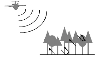
The backscattered waves can be considered as the sum of the three components in forest observations, as can be seen in Figure 1. In fact, the method proposed by (Freeman and Durden 1998) is the most popular technique in the scattering model decomposition, which can decompose the total power into surface (single-bounce) scattering (SB), double bounce scattering (DB), and volume scattering (VS) power.
Figure 1: Three scattering mechanisms (Mette 2007)
In the scattering model decomposition, the covariance matrix estimated by the PolSAR data is often used (Yamada, Onoda et al. 2008), which is defined by Equation 1.
C =< kk∗>
k = [SHH √ SHV Svv]t (Equation 1)
where < . > , * and t denote multilook processing, complex conjugate transpose and transpose, respectively. The decomposition model in Equation 1 is defined by
= + + � � (Equation 2)
where Cs, Cd and Cv are the basis of covariance matrices for the surface, double-bounce, and volume scattering components respectively. Power of each scattering component can be derived by the coefficient, fs, fd and fv.
Now assume that a set of PolInSAR data is available. In this case, two target vectors in their lexicographic form (kL1, kL2) are given by Equation 3, from two slightly different look angles.
k⃗ � = [S HH √ SHV Svv]t
k⃗ � = [S HH √ S HV Svv]t (Equation 3)
It is assumed that the covariance matrices of corresponding pair would be highly correlated. Thus they can be approximately modelled by Equation 4 (Yamada, Yamazaki et al. 2006, Yamada, Onoda et al. 2008, Minh, Zou et al. 2012).
= + + � �
= ��+ ��+ � � �� (Equation 4)
where �, � and �� are the interferometric phase to the corresponding component (Yamada, Onoda et al. 2008).
The outer products of the target vectors, provides three 3×3 complex matrices C11, C12 and C22 as follows,
[ ] = k⃗ � k⃗ � ∗
[ ] = k⃗ � k⃗ �∗
[ ] = k⃗ � k⃗ � ∗ (Equation 5)
C11 and C22 are the conventional Hermitian polarimetric covariance matrices, which describe the polarimetric properties for each individual image separately (Cloude 2008), while C12 is a matrix which contains polarimetric and interferometric information (Cloude 2008).
Again it is assumed that each component is mutually uncorrelated, thus the correlation matrix or interferometric matrix (C12), is decomposed to three scattering mechanisms (Yamada, Komaya et al. 2009, Minh and Zou 2013) i.e. SB, DB and VS1 (Equation 6).
= ��+ ��+ � � �� (Equation 6)
As discussed in (Yamada, Komaya et al. 2009), the three unknowns (phase parameters i.e. �, � and ��) are introduced for the interferometric phase and the number of additional equations are 4. As a result, 8 independent equations for 8 unknowns in C12 make the model-based decomposition for PolInSAR data solvable without any assumptions for and in the below components (Yamada, Komaya et al. 2009) (Equation 7):
[ ] = [| |
∗ ]
[ ] = [| |
∗ ] (Equation 7)
Since Cs and Cd have no volume related components, Cv and consequently ��can be easily estimated (Yamada, Komaya et al. 2009). This means that if the precise Cv is known, we can easily remove the volume scattering component from the original covariance matrices. Therefore, a General model for approximation of Cv is elaborated in the below subsection. 2.2 Covariance matrix of the volume component
Volume scattering is directly from the top layer of a forest. Several authors have argued that the scattering from a vegetation canopy can be reasonably represented by a cloud of randomly oriented infinitely thin cylinders (Freeman and Durden 1993, Yamaguchi, Moriyama et al. 2005). The scattering matrix of a vertically oriented elementary scatterer is expressed as Equation 8,
[ ] = [ ] (Equation 8)
1 Each component is fully described in Minh, N. P. and B. Zou (2013). "A
And when it is rotated by an angle � around the radar Line Of Sight (LOS), is generally expressed as Equation 9 (Arii, Van Zyl et al. 2010),
[ � ][ ][ −� ]
= [ + � � − �� �� � + �� � − � � − �� �� � − �� �]
(Equation 9)
in which, A= a+ b, B= a-b and C= 2c. Then the covariance matrix can be calculated as discussed in (Arii, Van Zyl et al. 2010). In fact, the nth power cosine-squared function (Equation 10) was used as a general distribution function in describing the general volume scattering component in this research. It is worth mentioning that the general distribution function expressed as a function of mean orientation angle of the elemental scatterers and its randomness (n) as follows.
�� �, � , = |{ − }
�|
∫ |{� − }�| (Equation 10)
in which, � is the mean orientation angle of the scattering elements and n represents the power of cosine-squared function. The randomness is decreased as n increases. The parameter n ranges from zero to infinity (Arii, van Zyl et al. 2011).
Since, this probability distribution function (pdf) determines the vegetation characteristics2, the usage of generalized probability density function based on the nth power of a cosine-squared function, which is characterized by two parameters (mean orientation angle and degree of randomness), makes this method useful for different vegetation types (Minh and Zou 2013).
By expanding the powers of sine and cosine, in calculated covariance matrix, it can be rewritten as a sum of three matrices (Equation 11),
[ �� � , ] = [ ] + + [ � ]
+ + − + [ � � ]
(Equation 11)
The basis covariance matrices in Equation 11, are expressed as (Arii, Van Zyl et al. 2010, Arii, van Zyl et al. 2011), Equation 12,
2 Freeman and Durden’s volume component can be described by the pdf of
uniform distribution. Additional information: Arii, M., J. J. Van Zyl and Y. Kim (2010). "A general characterization for polarimetric scattering from vegetation canopies." Geoscience and Remote Sensing, IEEE Transactions on 48(9): 3349-3357.
As mentioned before, the parameter n ranges from zero to infinity. However, there is little difference between distributions with values of n larger than about 20 or so (Arii, van Zyl et al. 2011). Therefore, the standard deviation (�) can be evaluated in terms of n as Equation 13, and it varies from range between 0 and 0.91.
� = √� + ∑ − ! ! !− ! −−�−�
= (Equation 13)
Using Equation 11 and 13, the general volume scattering model of (Equation 11) can be rewrite as there is no information available for randomness (�) and mean orientation angle (�). Thus, we should find a method for their estimation. In the below subsection the applied method for estimating the volume component is fully described.
� =
+� −√�⁄
[
√ ⁄
+�
− √ ⁄
√ ⁄ ]
(Equation 16)
where, = | ℎℎ| / | ��| . This volume scattering model ( � ) is called the reference volume scattering covariance matrix from now on.
This way, the best fit parameters of Equation 14 can be calculated using the reference volume scattering in Equation 16. In other words, the volume scattering covariance matrix is determined by varying randomness � and mean orientation angle � , so that �� � , � approximates to the � (Minh and Zou 2013). It is worth mentioning that, this step is repeated for each pixel in the image.
2.4 Phase and height estimation
When the generalized volume covariance matrix was estimated, the power of volume scattering component and also the canopy phase can be obtained by Equation 17,
��= |�| ��= � ,, (Equation 17)
In this stage, we can remove the volume scattering component from the original covariance matrices and a remainder matrix with four complex unknowns is presented as,
� = [ ] + [ � ] =
[| | � + | | �� � + ��
∗� + ∗�� � + �� ] (Equation 18)
In order to determine the above unknown parameters the modified ESPIRIT-based PolInSAR (Roy and Kailath 1989, Yamada, Sato et al. 2002, Guillaso, Reigber et al. 2005, Chen, Zhang et al. 2010) was employed and the parameters � , �� , , were determined as in (Minh and Zou 2013). Finally the argument of �� was chosen as the surface topography to be employed in the forest height estimation by Equation 19
ℎ�=��−�
� Equation 19
Where, ��, � , �� and ℎ� are vertical wavenumber, surface phase and canopy phase, respectively.
3. DATA AND EXPERIMENTAL RESULTS
Two different L-band datasets were used for the evaluation of the method, that are described with great detail in below subsections.
3.1 Simulated SAR data
The method was firstly evaluated by a simulated PolInSAR data of a forest, which was simulated by PolSARProSim software (Williams 2006), in L-band at 30 degree angle of incident. The stand height is 10m. The Pauli RGB image of the simulated data is presented in Figure 2.
Figure 2: Pauli image of the simulated SAR data
The calculated images of �� and � in the simulated data are presented in Figure 3.
a) b)
Figure 3: Estimated phase images; a) canopy phase, b) ground surface phase.
Finally the height map is presented as in Figure 4.
Figure 4: Height map of the simulated data
The height values were around 10 meters equal to the input simulated forest height.
3.2 Air-borne images
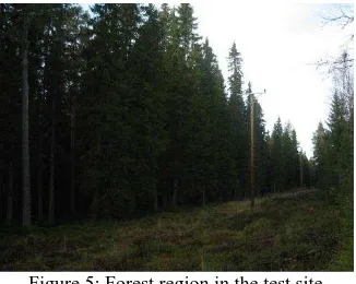
The BioSAR 2008 campaign has been intended to provide in support of decisions to be taken for the Earth Explorer Mission BIOMASS. The test site selected for the BioSAR 2008 campaign is the forested area within the Krycklan River catchment situated in Northern Sweden, which is about 50 km northwest of Umea. The dominating forest type is mixed coniferous. Figure 5 shows the test site.
Figure 5: Forest region in the test site
Sandberg et al. 2011). The characteristics of the used SAR images acquired in PolInSAR mode are as follows:
Table 1: Airborne data characteristics
Master image Slave image
Acquisition
date 14 October 2008 14 October 2008
Acquisition
time 11:25:22 11:42:03
Northing 64˚13’44” 64˚13’45”
Easting 19˚56’23” 19˚56’21”
Data Quicklook
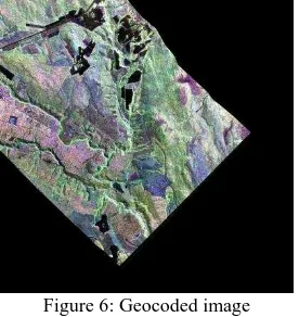
After estimation of height values for each image pixel, evaluation of the geocoded results was done using groundtruth data provided in the time of image acquisitions. Figure 6 and 7 represent the geocoded image and its regression analysis with measured heights, respectively.
Figure 6: Geocoded image
Number of plots which was used for evaluation of the results was about 36.
Figure 7: Regression line between the calculated and observed heights
4. CONCLUSION
Forest ecosystems play an important role in global change on the earth. Current concerns for ecosystem functioning require accurate biomass estimation and examination of its dynamics. Recently, there have been plenty of researches on the retrieval of forest height by single baseline PolInSAR. This paper aimed at the evaluation of a hybrid method in vegetation height estimation based on L-band multi-polarized air-borne SAR images in the campaign BioSAR 2008. The outcome of this study indicate that notwithstanding to the vegetation type, the forest height map can be calculated using the phase differencing method. Moreover, experimental results show the efficiency of the approach for vegetation height estimation in the test site.
However, as the objectives of the BioSAR 2008 campaign focused more on evaluating the effects of topography, it is recommended to investigate the topography of the test site in final estimated heights in our discussed phase difference method.
.
ACKNOWLEDGMENT
The author’s would like to thank BioSAR 2008 team for data provision.
REFERENCES
Antropov, O., Y. Rauste and T. Hame (2011). "Volume scattering modeling in PolSAR decompositions: Study of ALOS PALSAR data over boreal forest." Geoscience and Remote Sensing, IEEE Transactions on 49(10): 3838-3848.
Arii, M., J. J. Van Zyl and Y. Kim (2010). "A general characterization for polarimetric scattering from vegetation canopies." Geoscience and Remote Sensing, IEEE Transactions on 48(9): 3349-3357.
Arii, M., J. J. van Zyl and Y. Kim (2011). "Adaptive model-based decomposition of polarimetric SAR covariance matrices." Geoscience and Remote Sensing, IEEE Transactions on 49(3): 1104-1113.
Askne, J. I., P. B. Dammert, L. M. Ulander and G. Smith (1997). "C-band repeat-pass interferometric SAR observations of the forest." Geoscience and Remote Sensing, IEEE Transactions on 35(1): 25-35.
Bamler, R. and P. Hartl (1998). "Synthetic aperture radar interferometry." Inverse problems 14(4): R1.
Boscolo, M., M. Powell, M. Delaney, S. Brown and R. Faris (2000). "The cost of inventorying and monitoring carbon: lessons from the Noel Kempff climate action project." Journal of Forestry 98(9): 24-31.
Chen, J., H. Zhang and W. Chao (2010). Comparison between ESPRIT algorithm and three-stage algorithm for PolInSAR. Multimedia Technology (ICMT), 2010 International Conference on, IEEE.
Freeman, A. and S. L. Durden (1993). Three-component scattering model to describe polarimetric SAR data. San Diego'92, International Society for Optics and Photonics.
Freeman, A. and S. L. Durden (1998). "A three-component scattering model for polarimetric SAR data." Geoscience and Remote Sensing, IEEE Transactions on 36(3): 963-973.
Ghasemi, N., M. R. Sahebi and A. Mohammadzadeh (2013). "Biomass estimation of a temperate deciduous forest using wavelet analysis." Geoscience and Remote Sensing, IEEE Transactions on 51(2): 765-776.
Guillaso, S., A. Reigber and L. Ferro-Famil (2005). Evaluation of the ESPRIT approach in polarimetric interferometric SAR. Geoscience and Remote Sensing Symposium, 2005. IGARSS'05. Proceedings. 2005 IEEE International, IEEE.
Mette, T. (2007). Forest biomass estimation from polarimetric SAR interferometry, Technische Universität München.
Minh, N. P. and B. Zou (2013). "A Novel Algorithm for Forest Height Estimation from PolInSAR Image." International Journal of Signal Processing, Image Processing and Pattern Recognition 6(2): 15-32.
Minh, N. P., B. Zou and C. Yan (2012). Forest height estimation from PolInSAR image using adaptive decomposition method. Proc. 11th Int. Conf. Image Processing.
Roy, R. and T. Kailath (1989). "ESPRIT-estimation of signal parameters via rotational invariance techniques." Acoustics, Speech and Signal Processing, IEEE Transactions on 37(7): 984-995.
Tebaldini, S., M. M. d'Alessandro, H. T. M. Dinh and F. Rocca (2011). P band penetration in tropical and boreal forests: Tomographical results. Geoscience and Remote Sensing Symposium (IGARSS), 2011 IEEE International, IEEE.
Tebaldini, S. and F. Rocca (2009). "BioSAR 2008 Data Analysis II." ESTEC Contract No. 22052/08/NL/CT.
Treuhaft, R. N., S. N. Madsen, M. Moghaddam and J. J. Zyl (1996). "Vegetation characteristics and underlying topography from interferometric radar." Radio Science 31(6): 1449-1485.
Treuhaft, R. N. and P. R. Siqueira (2000). "Vertical structure of vegetated land surfaces from interferometric and polarimetric radar." Radio Science 35(1): 141-177.
Ulander, L. M. and J. Askne (1995). "Repeat-pass SAR interferometry over forested terrain." Geoscience and Remote Sensing, IEEE Transactions on 33(2): 331-340.
Ulander, L. M., G. Sandberg and M. J. Soja (2011). Biomass retrieval algorithm based on P-band biosar experiments of boreal forest. Geoscience and Remote Sensing Symposium (IGARSS), 2011 IEEE International, IEEE.
Van Zyl, J. J., Y. Kim and M. Arii (2008). Requirements for model-based polarimetric decompositions. Geoscience and Remote Sensing Symposium, 2008. IGARSS 2008. IEEE International, IEEE.
Williams, M. (2006). PolSARproSim Design Document and Algorithm Specification.
Yamada, H., R. Komaya, Y. Yamaguchi and R. Sato (2009). Scattering component decomposition for POL-InSAR dataset and its applications. Geoscience and Remote Sensing Symposium, 2009 IEEE International, IGARSS 2009, IEEE.
Yamada, H., H. Onoda and Y. Yamaguchi (2008). On scattering model decomposition with Pol-InSAR data. Synthetic Aperture Radar (EUSAR), 2008 7th European Conference on, VDE.
Yamada, H., K. Sato, Y. Yamaguchi and W. M. Boerner (2002). Interferometric phase and coherence of forest estimated by ESPRIT-based polarimetric SAR interferometry. Geoscience and Remote Sensing Symposium, 2002. IGARSS'02. 2002 IEEE International, IEEE.
Yamada, H., M. Yamazaki and Y. Yamaguchi (2006). "On Scattering model decomposition of PolSAR image and its application to the ESPRIT-based Pol-inSAR." EUSAR 2006.