Macro shocks and real stock prices
David E. Rapach*
Department of Economics and Finance, Albers School of Business and Economics, Seattle University, 900 Broadway, Seattle, WA 98122-4340, USA
Received 12 August 1999; received in revised form 18 January 2000; accepted 10 February 2000
Abstract
In this paper, I examine the effects of money supply, aggregate spending, and aggregate supply shocks on real US stock prices in a structural vector autoregression framework. Overall, the empirical results indicate that each macro shock has important effects on real stock prices. The real stock price impulse responses to the various macro shocks conform to the standard present-value equity valuation model, and they shed considerable light on the well-known negative correlation between real stock returns and inflation. An historical decomposition indicates that the late 1990s surge in real stock prices is due to a series of favorable structural shocks emanating from different sectors of the US economy. © 2001 Elsevier Science Inc. All rights reserved.
JEL classification: C32; E44; G12
Keywords: Real stock prices; Natural-rate hypothesis; Structural vector autoregression
1. Introduction
In addition to the idiosyncrasies of individual firms, general economic conditions are a key determinant of stock prices. In this paper, I use a structural vector autoregression (VAR) model to analyze the effects of money supply, aggregate spending, and aggregate supply shocks on the real value of a broad index of US stock prices. These macro shocks figure prominently in theoretical and empirical models of the macroeconomy and are generally regarded as important sources of fluctuations in aggregate real output, interest rates, and the
* Tel.:11-206-296-5705; fax:11-206-296-2486. E-mail address: [email protected] (D.E. Rapach).
price level. The primary objective of this paper is to measure the contribution made by these important macro shocks to real stock price fluctuations.
Following the methodology developed by Blanchard and Quah (1989), I rely on long-run restrictions to identify the macro shocks. More specifically, I use a set of long-run restrictions primarily motivated by the natural-rate hypothesis to identify money supply, aggregate spending, aggregate supply, and what I term “portfolio” shocks in a four-variable VAR in the price level, real stock prices, the interest rate, and real output. Since the natural-rate hypothesis is a standard feature of theoretical macro models, the identifying restrictions receive relatively wide theoretical support. Reliance on long-run identifying restrictions also leaves the short-run dynamics of the VAR unconstrained; theoretical models often have divergent short-run structures, suggesting that short-run restrictions are a less reliable source of identifying restrictions. Furthermore, long-run identifying restrictions often generate highly plausible dynamics in VAR models; see, for example, Keating (1992).
This paper is the first to use theoretically motivated restrictions to identify the effects of a set of important macro shocks on real stock prices in a VAR framework. Lee (1992) estimates a four-variable VAR in real stock returns, the real interest rate, industrial produc-tion growth, and inflaproduc-tion. Following the tradiproduc-tional VAR approach, he identifies a set of structural shocks by contemporaneously ordering the variables. This approach is tantamount to imposing a recursive contemporaneous structure—a structure which receives little theo-retical support—thus making it difficult to give a structural interpretation to the results reported in Lee (1992).1The theoretically motivated long-run restrictions used in the present paper are likely to be more successful in identifying the underlying structural shocks of economic interest. Lastrapes (1998) relies on theoretically motivated long-run restrictions based on the neutrality of money in order to identify the effects of money supply shocks in a VAR that includes real stock prices, the interest rate, and real output. Given his focus on liquidity effects, Lastrapes (1998) only identifies money supply shocks.2In the present paper, I also identify aggregate supply and aggregate spending shocks, as well as the portfolio shocks mentioned above. These nonmonetary macro shocks have potentially important effects on real stock prices, and analysis of these shocks is likely to be crucial for under-standing real stock price fluctuations.3
Overall, the structural VAR estimation results indicate that each macro shock has impor-tant effects on real stock prices. As in Lastrapes (1998), expansionary money supply shocks raise real stock prices and lower the interest rate in the short run. Money supply shocks also explain about a third of the variability in real stock prices at shorter horizons. Expansionary aggregate supply shocks raise real stock prices at both shorter and longer horizons. At longer horizons, aggregate supply shocks explain nearly 50% of the variability in real stock prices, indicating that the long-run productivity of the economy is the principal determinant of long-run changes in real stock prices. Expansionary aggregate spending shocks raise the interest rate and depress real stock prices over time. The estimation results also show that portfolio shocks (exogenous shocks to the demand for stocks) play an important role in determining real stock prices at shorter and longer horizons. The impulse responses of the endogenous variables in the VAR to each shock are highly plausible, suggesting that the long-run restrictions successfully identify the underlying structural shocks in the VAR.
price data. Firstly, there is the well-known negative correlation between real stock returns and inflation over the postwar period.4 The negative correlation has been considered anom-alous in that, as a claim to real assets, stocks should be a good hedge against inflation: Via a Fisher effect for equities, real stock returns should be unaffected by changes in inflation. The real stock price impulse responses to the various macro shocks generated by the structural VAR indicate that the negative correlation is explained by the concomitant impulse responses of the price level, the interest rate, and real output to the structural shocks. This lends support to the “proxy hypothesis” of Fama (1981). Another prominent feature of the data is the strong surge in real stock prices in the latter half of the 1990s. I use the structural VAR to perform an historical decomposition of real stock prices from the first quarter of 1995 through the first quarter of 1999. The historical decomposition indicates that aggregate supply and money supply shocks, as well as exogenous shifts by investors into stocks, are responsible for the sharp increase in real stock prices during this period.
The rest of the paper is organized as follows: Section 2 outlines the structural VAR model; Section 3 presents the estimation results, including impulse responses, forecast error variance decompositions, and the real stock price historical decomposition; Section 4 concludes.
2. The structural VAR model
Consider the following covariance-stationary VAR process, which can be viewed as the
reduced form of a general dynamic economic system:5
C~L!Dxt5et, (1)
where xtis an n-vector of endogenous variables (at time t) and, using the notation of Engle and Granger (1987), xt;I(1); L is the lag operator (that is, L s Þ0. By assuming that xt;I(1), shocks can have permanent effects on the levels of the
endogenous variables. The moving-average representation (MAR) for Dxt in terms of the
VAR shocks is obtained by inverting Eq. (1):
Dxt5D~L!et5
O
s50`
DsLset, (2)
where D(L) 5C(L)21 and D05In. The MAR describes the dynamic relationship between the endogenous variables and the VAR shocks. The VAR shocks are reduced-form shocks and therefore amalgams of the economically meaningful structural shocks. Assume that et5 Get, whereetis an n-vector of structural shocks.6Also assume that E(ete9t)5 Seis diagonal.
This is a reasonable assumption if the structural shocks emanate from distinct sectors of the economy. A convenient normalization sets the main diagonal ofSeto unity, so thatSe5In.
7
following Blanchard and Quah (1989). In the next section, I estimate Eq. (1) with xt5(pt, st, it, yt)9, where ptis the price level, stis the real price of stocks, itis the nominal interest rate, and yt is real output. All variables except the nominal interest rate are in log-levels. Appendix 1 explains how a set of six restrictions on the long-run response of xt to the structural shocks can be used to identify four structural shocks. The six restrictions take the following form, expressed below in terms of the matrix of long-run multipliers (H):
lim
where eMS,t,ePO,t,eIS,t, andeAS,tare money supply, portfolio, aggregate spending (IS), and
aggregate supply shocks, respectively. The six restrictions are h215h315h415h425h43
50 and h325zh22, where z is a constant. 9
The h21 5 h31 5 h41 5 0 restrictions imply that money supply shocks—permanent
exogenous changes in the level of the money supply— have no long-run effect on real stock prices, the interest rate, or real output. The long-run structure does allow for an expansionary money supply shock to increase the price level in the long run. The structural VAR is thus characterized by long-run monetary neutrality, a standard result in monetary theory.10The
h42 5 h43 5 0 restrictions mean that portfolio and aggregate spending shocks have no
long-run effect on real output. Taken together with the h4150 restriction, these restrictions impose the natural-rate hypothesis: Only aggregate supply shocks—such as oil price and technology shocks that alter potential output—affect the long-run level of real output. As noted in the introduction, the natural-rate hypothesis is a standard feature of theoretical macro models.11
The portfolio shock represents an exogenous shock to the demand for stocks, in the context of the three-asset model of Tobin (1969). This shock could result, for example, from a change in transaction costs in the stock market or an exogenous change in the perceived riskiness of stocks (an “equity-premium” shock). This is a pure portfolio shock, so it does not affect potential output (h4250). However, it likely will affect the interest rate: An exogenous shift toward stocks requires a decrease in the price of bonds (an increase in the interest rate) for asset market equilibrium to obtain. With an assumed value for z, the h32 5 zh22 restriction establishes the long-run interest rate response to a portfolio
shock. In the benchmark VAR model, I assume that z 5 0.025. This means that a 20%
permanent increase in real stock prices resulting from an exogenous portfolio shift into stocks requires a 0.5 percentage point long-run increase in the interest rate in order to maintain asset market equilibrium. Below, I examine the sensitivity of the estimation results to variations in z.12It is important to note that under the particular long-run structure assumed here, the dynamic effects of money supply and aggregate supply shocks on the endogenous variables are not affected by changes in z.13Thus, a number of key inferences are invariant to the assumed value of z.
run (h4350) and permanently increases the interest rate. These are standard predictions in aggregate-demand-aggregate-supply models.
In summary, I identify the effects of money supply, portfolio, aggregate spending, and aggregate supply shocks on the price level, real stock prices, the interest rate, and real output through run restrictions primarily motivated by the natural-rate hypothesis. The long-run restrictions appear to comprise a relatively uncontroversial set of identifying restrictions. As noted above, an important advantage of this identification strategy is that, unlike the traditional VAR approach, it leaves the short-run dynamics of the VAR unconstrained.
While long-run identifying restrictions are theoretically appealing, Faust and Leeper (1997) point to potential problems relating to the use of infinite-horizon identifying restric-tions. Two of the potential problems involve confounding the effects of different structural shocks. These problems appear most serious for bivariate VARs and data sampled at relatively low frequencies. Given that I identify four structural shocks and use quarterly data, these problems are unlikely to be serious for the present application. A third potential problem is that results based on infinite-horizon identifying restrictions may be unreliable for a finite sample. In order to examine the relevance of this potential problem for the present application, I follow Lastrapes (1998) and reestimate the structural VAR with the identifying restrictions imposed at long but finite horizons.
3. Estimation results
The quarterly data for this study span 1959:3–1999:1. The price level (pt) is the implicit GDP deflator. The S&P 500 index deflated by the implicit GDP deflator serves as the real stock price measure (st). The nominal interest rate (it) is the 3-month Treasury bill rate
(secondary market).14 Real output is GDP in constant 1992 dollars (yt). The data are
described in more detail in Appendix 2. Recall that all variables except the nominal interest rate are in log-levels.
Standard unit root tests cannot reject the null hypothesis that each endogenous variable— pt, st, it, yt—is nonstationary, indicating that xt;I(1).
15
Sequential testing using the modified likelihood ratio statistic of Sims (1980) and considering a maximum lag order of eight selects a VAR(7) [p57 in Eq. (1)]. Ljung-Box Q statistics give no indication of serial correlation in any of the VAR equations for the VAR(7) specification. After allowing for differencing and lags, there are 151 observations (1961:3–1999:1).16The structural shocks are identified using the long-run restrictions described in the previous section.
3.1. Impulse response and variance decomposition analysis
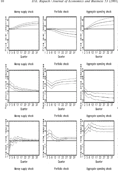
line with standard stories of the monetary transmission mechanism that rely on some form of nominal stickiness. The money supply shock also brings about a short-run increase in real stock prices, which is easily explained by the standard present-value equity valuation model: The increase in real output increases anticipated short-run real earnings, while the decrease in the interest rate decreases the rates at which future cash flows are discounted.19Lastrapes (1998) also finds that an expansionary money supply shock lowers the interest rate and increases real stock prices in the short run.20
The second column of Fig. 1 contains the impulse responses to a portfolio shock. In terms of the present-value equity valuation model, this shock can be viewed as an exogenous decrease in the equity-risk premium component of the discount rate for equity cash flows. Real stock prices increase sharply in the short run in response to the portfolio shock. Not surprisingly, the interest rate increases (bond prices fall) in response to this exogenous portfolio shift into stocks. Interestingly, real output falls after a number of quarters. This may result from the increase in the interest rate, which lowers aggregate demand and thus real output with a lag. The eventual fall in the price level supports this interpretation. The decline in real output may also be partly explained by an endogenous Federal Reserve response to the portfolio shock. The Fed may follow a tight monetary policy in response to the jump in stock prices, concerned that the stock market is “overvalued.”21
The impulse responses to an expansionary aggregate spending shock are found in the third column of Fig. 1. In response to the aggregate spending shock, the price level and interest rate increase over time to permanently higher levels, and there is a temporary increase in real output. These impulse responses again accord well with standard macro theory, and the real stock price impulse response is again in line with the present-value equity valuation model. Real stock prices change relatively little in the immediate quarters after the shock: While the increase in real output raises anticipated real earnings in the short run, the concomitant increase in the interest rate causes these earnings to be discounted at a higher rate. Real stock prices eventually decrease since the increase in real output and earnings is only temporary while the increase in the interest rate is permanent.
As expected, an expansionary aggregate supply shock brings about short-run and perma-nent decreases in the price level and short-run and permaperma-nent increases in real output (see the fourth column of Fig. 1). The shock also decreases the interest rate, especially at shorter horizons. Again, the present-value equity valuation model can account for the real stock price impulse response: permanently higher real output levels generate permanently higher real earnings and thus permanently higher real stock prices; the lower interest rate also lifts real stock prices.
period as real output moves to a permanently higher level. The increase in real output boosts real stock prices as expectations of real earnings are adjusted upward. This, of course, is the “proxy hypothesis” of Fama (1981): Inflation and real activity are negatively related while real activity and real stock returns are positively related.
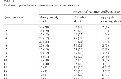
While aggregate supply shocks are clearly an important source of the negative real stock price growth-inflation correlation, the impulse responses to money supply and aggregate spending shocks at intermediate horizons are also not inconsistent with a negative real stock price growth-inflation correlation. Looking back to the first column of Fig. 1, the peak real output response to a money supply shock occurs in the sixth quarter; after this, real output growth is typically below its trend as output adjusts back to its potential level. The price level, on the other hand, continues to increase after the sixth quarter to a permanently higher level; inflation will thus be above trend and real output growth below trend for a number of quarters. Real stock price growth jumps in the first two quarters in response to the short-run increase in real output growth and decrease in the interest rate. However, real stock price growth is below trend by the third quarter as the reverse in real output growth nears and the interest rate begins rising back to its original level. From the third quarter on, a negative correlation between real stock price growth and inflation is generated by the money supply shock as the economy moves to a new long-run equilibrium. A similar pattern can be observed for the aggregate spending shock: The interest rate increases and inflation is above trend, while real output and real stock price growth are below trend, for a number of quarters as the economy approaches a new long-run equilibrium. These adjustments to new long-run equilibria also help explain why stock prices sometimes fall in response to good economic news; see Cogley (1996). If the source of an increase in real output is an aggregate demand shock, then good news about real output growth will soon signal that the economy is overheated. This portends higher inflation and interest rates and lower real output and earnings levels. According to the present-value equity valuation model, real stock prices fall. The real stock price forecast error variance decompositions, reported in Table 1, convey the essentially same information as the real stock price impulse responses, but in a different form. At shorter horizons, portfolio shocks explain most of the variability in real stock prices, followed by money supply shocks. Given that money is neutral in the long run, the importance of money supply shocks in determining short-run real stock prices indicates that
real stock prices have an important temporary component.22 At intermediate horizons,
money supply shocks and portfolio shocks begin to diminish, while aggregate supply shocks grow, in importance. At longer horizons, aggregate supply shocks are the leading determi-nant of the variability in real stock prices (nearly 50%). This indicates that the underlying productive potential of the economy is the principal determinant of the long-run level of real stock prices.
3.2. Sensitivity analysis
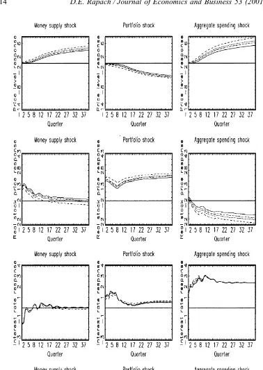
16, 28, and 40 quarters are given in Fig. 2. The impulse responses are very robust to imposing the identifying restrictions at long but finite horizons (especially 28 and 40 quarters).23This indicates that the estimation results for the benchmark structural VAR do not depend critically on imposing identifying restrictions at the infinite horizon.
I next explore the sensitivity of the estimation results to changes in z, where z determines the long-run interest rate response to a portfolio shock. Recall that z50.025 is assumed for the benchmark structural VAR. Fig. 3 presents the impulse responses to the portfolio and aggregate spending shocks for different z values. As noted above, the impulse responses to the money supply and aggregate supply shocks are invariant to the assumed z value. Fig. 3 shows that the impulse responses to the portfolio and aggregate spending shocks are largely unaffected by assuming different z values. Note that the real stock price response to a portfolio shock is typically smaller (larger), while the response to an aggregate spending shock is larger (smaller), in absolute value, when z50.05 (z50.01) than in the benchmark
structural VAR where z 50.025.
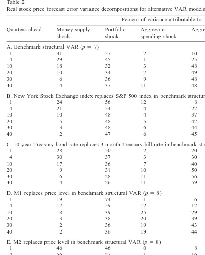
I estimated a number of other alternative structural VARs to further examine the sensi-tivity of the results of the benchmark structural VAR. The results are given in the form of real stock price variance decompositions in Table 2. First, I replaced the S&P 500 stock price index with the New York Stock Exchange index in the benchmark structural VAR. The results change little. Next, I replaced the 3-month Treasury bill rate with the 10-year
Table 1
Real stock price forecast error variance decompositions
Percent of variance attributable to:
Fig. 3. Impulse responses to one-standard-deviation (unit) structural shocks for different z values. Note: Solid lines correspond to z50.025; short dashed lines correspond to z50.01; long dashed lines correspond to z5
Table 2
Real stock price forecast error variance decompositions for alternative VAR models
Percent of variance attributable to:
A. Benchmark structural VAR (p57)
1 31 57 2 10
B. New York Stock Exchange index replaces S&P 500 index in benchmark structural VAR (p55)
1 24 56 12 8
C. 10-year Treasury bond rate replaces 3-month Treasury bill rate in benchmark structural VAR (p53)
1 28 50 2 20
D. M1 replaces price level in benchmark structural VAR (p58)
1 19 74 1 6
E. M2 replaces price level in benchmark structural VAR (p58)
1 46 46 0 8
F. Real oil price added to benchmark structural VAR (p55)
1 20 59 5 14 (nonoil price), 2 (oil price)
Treasury bond rate in the benchmark structural VAR. Again, the results for this VAR are similar to those of the benchmark model, although aggregate supply shocks account for nearly 60% of the variability in real stock prices at longer horizons in this alternative structural VAR (compared to nearly 50% in the benchmark structural VAR). Replacing the price level with the M1 monetary aggregate changes the results relatively little. Replacing the price level with the M2 monetary aggregate increases the importance of money supply shocks (at the expense primarily of portfolio shocks) in explaining real stock price variability at all reported horizons compared to the benchmark structural VAR. Finally, I also estimated a structural VAR that adds the real price of oil as an endogenous variable to the benchmark structural VAR, so that xt5(pt, st, it, yt, ot)9, where otis the real price of oil (in log-levels). This allows the supply shock to be divided into oil price and nonoil price components, as in Fackler and McMillin (1998). Identification is achieved in this VAR by additionally assum-ing that money supply, portfolio, aggregate spendassum-ing, and aggregate nonoil price supply shocks have no long-run effect on the real price of oil (that is, the real price of oil is exogenous in the long run).24 The results are similar to those of the benchmark structural VAR in terms of the relative importance of money supply, portfolio, aggregate spending, and aggregate supply shocks. Interestingly, oil price shocks individually account for much of the variability in real stock prices at longer horizons. Insofar as this structural VAR correctly separates nonoil price and oil price aggregate supply shocks, this suggests that oil price shocks have been an especially important aggregate supply shock in determining real stock prices during the postwar era.25
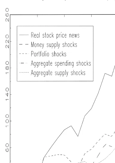
3.3. Real stock price historical decomposition
In this section, I use the benchmark structural VAR model to identify the sources of fluctuations in real stock prices during the late 1990s. The solid line in Fig. 4 displays the fluctuations in real stock prices from 1995:1–1999:1 that could not be predicted using the VAR and data through 1994:4. These movements in real stock prices are labeled “news.” The other lines show the part of the news that is accounted for by each structural shock.
Fig. 4 shows that real stock prices are much higher in 1999:1 than could have been predicted from the VAR through 1994:4. Expansionary aggregate supply shocks account for most of the increase in real stock prices. This suggests that the late 1990s surge in real stock prices is due in large part to growth in the potential output of the US economy. Expansionary money supply shocks have also helped boost real stock prices, while aggregate spending shocks have had very little influence on real stock prices, during the late 1990s. The part of the increase in real stock prices due to expansionary money supply shocks is not sustainable, since money supply shocks are assumed to have no long-run effect on real stock prices.
Exogenous shifts into stocks on the part of investors also account for much of the increase in real stock prices during the late 1990s. This supports the view of Carlson and Sargent (1997), who argue that the ascent in stock prices in the late 1990s cannot be explained by projected earnings growth alone and suggest a decline in the equity premium resulting from a focus on long-horizon returns. This shift in focus corresponds to a portfolio shock in the present model.
surge in real stock prices is the result of a series of favorable structural shocks emanating from different sectors of the US economy.
4. Conclusion
In this paper, I have relied on theoretically motivated long-run restrictions in a VAR model to identify the effects of a set of important macro shocks on real stock prices. The estimated impulse responses of all of the endogenous variables in the VAR—the price level, real stock prices, the interest rate, and real output—to money supply, portfolio, aggregate spending, and aggregate supply shocks are highly plausible, suggesting that the long-run identification strategy successfully identifies the macro shocks in the VAR. Each macro shock appears to have important effects on real stock prices, and the real stock price impulse responses are well explained by the standard present-value equity valuation model. Aggre-gate supply shocks appear especially important in explaining fluctuations in real stock prices at longer horizons, indicating that the productive potential of the economy is the key determinant of low-frequency movements in the real value of equities. The concomitant impulse responses of the endogenous variables to each macro shock help explain the well-known negative correlation between real stock returns and inflation in postwar data. Finally, an historical decomposition of real stock prices points to expansionary aggregate supply and money supply shocks, as well as exogenous portfolio shifts into stocks by investors, as the forces behind the surge in real stock prices in the late 1990s.
Notes
1. See the criticism of the traditional VAR approach in Cooley and LeRoy (1985). 2. That is, Lastrapes (1998) leaves the complete set of structural shocks underidentified,
but imposes enough restrictions to identify money supply shocks.
3. Another class of extant studies estimates the effects of monetary and/or fiscal policy shocks on real stock returns by regressing real stock returns on measures of monetary and/or fiscal policy shocks; see, for example, Davidson and Froyen (1982), Sorensen (1982), McMillin and Laumas (1988), and Darrat (1988). Such single-equation real stock return regression models are likely to be plagued by misspecification and simultaneity problems.
4. Early studies finding a negative correlation include Bodie (1976), Jaffe and Man-delker (1976), Nelson (1976), and Fama and Schwert (1977).
5. An intercept term is suppressed without loss of generality.
6. Since E(et) 50 and E(ete9t2s) 50 for all sÞ0, E(et) 50 and E(ete9t2s) 50 for all s Þ0.
7. This normalization does not affect the generality of the results. For example, the main diagonal of G could instead be set to unity.
9. The following discussion assumes that the elements of the main diagonal of H are positive. This holds for the structural VAR estimated below in Section 3.
10. I am implicitly assuming that the long-run increase in ptequals the long-run exoge-nous increase in the log-level of the money supply. Note that under the assumptions that pt;I(1) and actual and expected inflation coincide in the long run, changes in the long-run nominal and real interest rates are equivalent since Dpt;I(0) (that is, there are no permanent changes in the inflation rate). The h3150 restriction can thus be interpreted as requiring that money supply shocks have no long-run effect on the real, as well as the nominal, interest rate.
11. Any potential long-run real output effect associated with money supply, aggregate spending, and portfolio shocks is considered to be of second-order importance. See the discussion of the long-run effects of aggregate demand shocks on real output in Blanchard and Quah (1989).
12. Cogley (1993) follows a similar identification strategy in a structural VAR frame-work. That is, he allows a parameter to take on a nonzero value in order to achieve identification. He then examines the sensitivity of the results to variations in the parameter. Note that I only choose h32to be proportional to h22in order to generate a long-run interest rate response that seems plausible given the long-run increase in real stock prices. I could simply have set h32equal to a constant, but it is difficult to choose a plausible value for h32 in isolation from the long-run real stock price response.
13. The identified values of h11, h14, h24, h34and h44do not depend on the assumed value of z in Eq. (3).
14. This is the most commonly used measure of the interest rate in extant studies. 15. The standard tests are the augmented Dickey and Fuller (1979) and Phillips and
Perron (1988) tests, which treat nonstationarity as the null hypothesis (and stationarity as the alternative). The unit root tests of Kwiatkowski et al. (1992, KPSS) treat stationarity as the null hypothesis (and nonstationarity as the alternative). The null hypothesis of stationarity is easily rejected using KPSS tests for pt, st, it, and yt, further indicating that these variable are nonstationary. Standard tests also overwhelmingly reject the null hypothesis thatDst,Dit, orDytis nonstationary, and KPSS tests cannot reject the null hypothesis thatDst, Dit, or Dytis stationary, indicating that st, it, and yt are I(1). While the null hypothesis thatDptis nonstationary is also rejected in a number of cases using the standard tests, the results are more mixed than forDst,Dit, andDyt. The results are also more mixed using the KPSS tests. (The complete unit root test results are available upon request from the author.) I follow Lee (1992) and Lastrapes (1998) by treating ptas I(1). I discuss the estimation results for a model with nonstationary inflation [pt; I(2) orDpt; I(1)] in footnote 25 below.
How-ever, the Monte Carlo evidence in Miyao (1996) suggests that, unlike the Engle-Granger test, the Johansen test often has a true size that is considerably larger than the nominal size. (The complete cointegration test results are available upon request from the author.)
17. Since the variances of the structural shocks are normalized to one, these are the impulse responses to unit structural shocks. To get a feel for sampling error, standard-error bands are obtained through 1,000 bootstrap replications.
18. I also computed the real interest rate response to each structural shock using actual future inflation as a proxy for expected inflation [as in Galı´ (1992)]. The nominal and real interest rate responses to each shock follow similar patterns, so that the descrip-tion of the nominal interest rate response to each shock typically applies to the real interest rate response as well.
19. The present-value equity valuation model can be expressed as:
St5Et
O
where St is the real price of stocks; Et is the expectations operator conditional on information available at time t; Rtis the real rate at which cash flows are discounted
(the sum of the risk-free bond rate and an equity-risk premium); Dt is the real
dividend.
20. Lastrapes (1998) argues that these effects need to be accounted for in any successful theory of the business cycle. Insofar as money directly affects real stock returns, he interprets the positive real stock price response to an expansionary money supply shock as evidence against limited-participation models which posit tight institutional links between bond markets and the money supply process. The price level appears sticky in limited-participation models, even though it is flexible, since it does not adjust completely to a money supply shock in the short run due to financial market frictions. [See Christiano and Eichenbaum (1992) and Fuerst (1992) for examples of limited-participation models.] Christiano et al. (1997) find that when sticky-price models are calibrated to produce a plausible liquidity effect, they also produce the counterfactual result that profits fall in response to an expansionary money supply shock. While a limited-participation model is capable of generating a delayed price level response and a plausible liquidity effect, they find that it can also generate an increase in profits in response to an expansionary money supply shock. Christiano et al. (1997) construe this as evidence against the sticky-price model and in favor of the limited-participation model. To the extent that the increase in real stock prices reflects increases in profits, the impulse responses to a money supply shock in Fig. 1 can also be construed as evidence in support of the limited-participation model.
21. Irrational exuberance?
22. This point is made by Lastrapes (1998).
at a horizon, say, of 28 quarters does not impose long-run neutrality in a strict sense since the responses beyond 28 quarters are not restricted to be zero. However, especially when the restrictions are imposed at 28 and 40 quarters, the impulse responses for the variables that are restricted to zero do not stray far from zero after they reach the horizon at which the restriction is imposed.
24. Fackler and McMillin (1998) use a similar identification scheme.
25. I also estimated the benchmark structural VAR using a sample truncated at 1981:4 in order to examine the sensitivity of the results to the long bull market of 1982–1999. Of course, this sample eliminates almost half of the available observations and the estimates are therefore much less precise. The most notable differences between the results for the truncated sample and the results for the full sample are that money supply shocks account for less of real stock price variability at shorter horizons, while portfolio shocks (aggregate supply shocks) account for more (less) of real stock price variability at longer horizons. I also estimated a structural VAR where the price level is treated as I(2) or, in other words, inflation is nonstationary [Dpt;I(1)]. In terms of identification,Dpt1kreplaces pt1kand h31is restricted to equal h11instead of zero in Eq. (3). The model with nonstationary inflation thus assumes long-run monetary superneutrality. The most notable differences between the results for this structural VAR and those of the full-sample benchmark structural VAR are the following: Money supply shocks account for very little of the variability in real stock prices at shorter horizons; supply shocks account for less of real stock price variability at longer horizons; aggregate spending shocks are more important at all horizons in determining real stock prices. Note that long-run monetary superneutrality receives far less theoretical support than long-run monetary neutrality; see the survey in Orphanides and Solow (1990). I leave further consideration of the model with nonstationary inflation to future research.
26. Note that C(1)5 In 2C1 2C2 2. . . 2Cp.
27. Of course, this is only a necessary condition for identification since the system of equations defined by Eq. (13) may not have a solution. This condition is akin to the order condition in classical simultaneous equations estimation.
28. The k-period-ahead forecast error for xtin terms of the structural shocks is given by
S
k-period-ahead forecast error variance for the ith variable is therefore
S
piw,s!2. Finally, the percentage of the k-period-ahead forecast error
variance for the ith variable attributable to the jth structural shock is given by:
Acknowledgments
The author thanks Alan Isaac, Barry Pfitzner, Mark Wohars, and especially two anony-mous referees for very helpful comments on earlier drafts. The usual disclaimer applies.
Appendix 1. Identification of the structural shocks
Recall the VAR process, Eq. (1), and its associated MAR, Eq. (2). The dynamic effects of the VAR shocks on Dxtare given by:
The MAR for the levels of xtin terms of the VAR shocks is given by:
xt5~12L!21D~L!e
so that the dynamic effects of the VAR shocks on xtare given by:
x
Observe that the long-run effects of the VAR shocks on xtcan be expressed as:26
lim
As discussed in the text, the VAR shocks are reduced-form shocks and therefore amal-gams of the underlying structural shocks. Recall that et5 Get, where et is an n-vector of structural shocks. Also recall the assumption that E(e
te9t)5 Seis diagonal and the convenient
normalization that sets the main diagonal ofSeequal to unity (Se5In). The MAR for Dxtin terms of the structural shocks is given by:
Dxt5D~L!Ge
so that the dynamic effects of the structural shocks on Dxtcan be expressed as:
Dx
xt5~12L!21D~L!Ge
so that the dynamic effects of the structural shocks on xtare given by:
x
The long-run effects of the structural shocks on xtare given by:
lim
Note that H is the matrix of long-run multipliers for the endogenous variables with respect to the structural shocks: hijgives the infinite-horizon response of the ith endogenous variable to the jth structural shock. The long-run structure of the model can also be described by
lim k3`
xt1k 5 Het.
I identify the structural shocks by relying on long-run restrictions. Since et 5 Get and
Se5In, Se5GG9. Using G 5C(1)H from Eq. (12),
C~1!21S eC~1!
2195
HH9. (13)
OLS estimation of Eq. (1) provides consistent and efficient estimates of C(L) andSeand thus of the left-hand-side of Eq. (13). The left-hand-side of Eq. (13) is symmetric and has n(n1
1)/2 unique elements, while the right-hand-side has n2 unknowns (the n2 elements of H). Imposing n(n21)/2 restrictions on the long-run multiplier matrix H allows H to be identified from the system of n(n 11)/2 unique equations defined by Eq. (13).27 With H in hand, G is identified [recall that G 5 C(1)H]. The impulse responses of the variables in xt to the structural shocks are calculated through Eq. (11); the forecast error variance decompositions of the variables in xtin terms of the structural shocks can be calculated using Eq. (10).
28 For the model estimated in the text, xt5(pt, st, it, yt)9, so that n 54 and n(n 21)/256. The six long-run restrictions used to identify the four structural shocks are given in Eq. (3): h215 h315 h415h425h43 50, h325 zh22.
Appendix 2. Data
The data are from the Federal Reserve Economic Database (FRED) and Global Financial Data. Details for each time series are given below.
Price Level GDP implicit price deflator (FRED series GDPDEF), 19925100. The series is quarterly and seasonally adjusted.
Real Stock Prices S&P 500 nominal stock price index (Global Financial Data series
stock price index series is monthly. Quarterly observations are obtained by averaging over the three months comprising each quarter.
3-month Treasury Bill Rate This is the secondary market rate (FRED series TB3MS).
The original series is monthly. Quarterly observations are obtained by averaging over the three months comprising each quarter.
Real GDP GDP in billions of fixed 1992 dollars at an annual rate (FRED series GDP92).
The series is quarterly and seasonally adjusted.
References
Bernanke, B.S. (Autumn 1986.) Alternative explanations of the money-income correlation. Carnegie-Rochester Conference Series on Public Policy 25:49 –100.
Blanchard, O.J., & Quah, D. (Sep. 1989.) The dynamic effects of aggregate demand and supply disturbances. American Economic Review 79 (4):655– 673.
Bodie, Z. (May 1976.) Common stocks as a hedge against inflation. Journal of Finance 31 (2): 459 – 470. Carlson, J.B., & Sargent, K.H. (Quarter 2 1997.) The recent ascent of stock prices: Can it be explained by earnings
growth or other fundamentals? Federal Reserve Bank of Cleveland Economic Perspectives 33 (2):2–12. Christiano, L.J., & Eichenbaum, M. (May 1992.) Liquidity effects and the monetary transmission mechanism.
American Economic Review 82 (2):346 –353.
Christiano, L.J., et al. (June 1997.) Sticky price and limited participation models: A comparison. European Economic Review 41 (6):1201–1249.
Cogley, T. (May 1993.) Empirical evidence on nominal wage and price flexibility. Quarterly Journal of Economics 108 (2):475– 491.
Cogley, T. (Dec. 1996.) Why do stock prices sometimes fall in response to good economic news? Federal Reserve Bank of San Francisco Economic Letter 96 (36).
Cooley, T.F., & LeRoy, S.F. (Nov. 1985.) Atheoretical macroeconomics: A critique. Journal of Monetary Economics 16 (3):283–308.
Darrat, A.F. (Aug. 1988.) On fiscal policy and the stock market. Journal of Money, Credit, and Banking 20 (3):353–363.
Davidson, L.S., & Froyen, R.T. (March 1982.) Monetary policy and stock returns: Are stock markets efficient? Federal Reserve Bank of St. Louis Review 64 (3):3–12.
Dickey, D.A., & Fuller, W.A. (June 1979.) Distribution of the estimators for autoregressive time series with a unit root. Journal of the American Statistical Association 74 (366):427– 431.
Engle, R.F., & Granger, C.W.J. (March 1987.) Co-integration and error correction: Representation, estimation, and testing. Econometrica 55 (2):251–276.
Fackler, J.S., & McMillin, W.D. (Jan. 1998.) Historical decomposition of aggregate demand and supply shocks in a small macro model. Southern Economic Journal 64 (3):648 – 664.
Fama, E.F. (Sep. 1981.) Stock returns, real activity, inflation, and money. American Economic Review 71 (4):545–565.
Fama, E.F., & Schwert, G.W. (Nov. 1977.) Asset returns and inflation. Journal of Financial Economics 5 (2):115–146.
Faust, J., & Leeper, E. (July 1997.) When do long-run identifying restrictions give reliable results? Journal of Business and Economic Statistics 15 (3):345–353.
Fuerst, T.S. (Feb. 1992.) Liquidity, loanable funds, and real activity. Journal of Monetary Economics 29 (1):3–24. Galı´, J. (May 1992.) How well does the IS-LM model fit postwar US data? Quarterly Journal of Economics 107
(2):709 –738.
Johansen, S. (June/Sep. 1988.) Statistical analysis of cointegration vectors. Journal of Economic Dynamics and Control 12 (2/3):231–254.
Keating, J.W. (Sep./Oct. 1992.) Structural approaches to vector autoregressions. Federal Reserve Bank of St. Louis Review 74 (5): 37–57.
Kwiatkowski, D., et al. (Oct.-Dec. 1992.) Testing the null hypothesis of stationarity against the alternative of a unit root. Journal of Econometrics 54 (1–3):159 –178.
Lastrapes, W. D. (June 1998.) International evidence on equity prices, interest rates and money. Journal of International Money and Finance 17 (3):377– 406.
Lee, B.-S. (Sep. 1992.) Causal relations among stock returns, interest rates, real activity, and inflation. Journal of Finance 47 (4):1591–1603.
McMillin, W.D., & Laumas, G.S. (March 1988.) The impact of anticipated and unanticipated policy actions on the stock market. Applied Economics 20 (3):377–384.
Miyao, R. (Aug. 1996.) Does a cointegrating M2 demand relation really exist in the United States? Journal of Money, Credit, and Banking 28 (3):365–380.
Nelson, C.R. (May 1976.) Inflation and rates of return on common stocks. Journal of Finance 31 (2):471– 483. Orphanides, A., & Solow, R.M. (1990.) Money, inflation, and growth. In Handbook of Monetary Economics
(B.M. Friedman and F.H. Hahn, eds.). New York: North-Holland, pp. 223–261.
Phillips, P.C.B., & Perron, P. (June 1988.) Testing for a unit root in time series regression. Biometrika 75 (2):335–346.
Sims, C.A. (Jan. 1980.) Macroeconomics and reality. Econometrica 48 (1):1– 48.
Sims, C.A. (Winter 1986.) Are forecasting models usable for policy analysis? Federal Reserve Bank of Minneapolis Quarterly Review 10 (1):2–16.
Sorensen, E.H. (Dec. 1982.) Rational expectations and the impact of money upon stock prices. Journal of Financial and Quantitative Analysis 17 (5):649 – 662.