www.elsevier.com / locate / econbase
Econometric applications of high-breakdown robust regression
techniques
a b c ,
*
Asad Zaman , Peter J. Rousseeuw , Mehmet Orhan
aLahore University of Management Science, Lahore, Pakistan b
Department of Mathematics and Computer Science, Universitaire Instelling Antwerpen (UIA), Antwerp, Belgium c
Department of Economics and Computer Science, Fatih University, Istanbul, Turkey Received 13 March 2000; accepted 15 July 2000
Abstract
A literature search shows that robust regression techniques are rarely used in applied econometrics. We present a technique based on Rousseeuw and Van Zomeren [Journal of the American Statistical Association, 85 (1990) 633–639] that removes many of the difficulties in applying such techniques to economic data. We demonstrate the value of these techniques by re-analyzing three OLS-based regressions from the literature.
2001 Elsevier Science B.V. All rights reserved.
Keywords: High breakdown estimates; Masking; Robust regression; Outlier; Leverage point; Least trimmed squares (LTS); Minimum covariance determinant (MCD)
JEL classification: C2; C52
1. Introduction
Since it is well-established that even high quality data tend to contain outliers, and it is a rare economic data set that qualifies as ‘high-quality’, one would expect far greater reliance on robust regression techniques than is actually observed. Searching through ECONLIT for the term ‘robust regression’ led to a remarkably low total of 14 papers published in different journals most of which apply robust regression techniques to real economic data sets. We believe that this reluctance to use robust regression techniques may be due to the following factors.
• The belief that large sample sizes make robust techniques unnecessary — with enough data, one can find the truth.
*Corresponding author. Tel.: 190-212-889-0810; fax: 190-212-889-0832.
E-mail address: [email protected] (M. Orhan).
• The belief that outliers can be detected simply by eye, or by looking for unusual OLS residuals, or by sensitivity analysis, obviating the need for a robust analysis.
• Existence of several ‘robust regression’ techniques with little guidance available as to which is appropriate.
• Unfamiliarity with interpretation of results from a robust analysis.
• Unawareness of gains available from robust analysis in real data sets.
In this paper we hope to remove some of these barriers and facilitate more routine use of a particular set of robust regression procedures, based on Rousseeuw and Van Zomeren (1990) and modern algorithms. We comment on the factors listed above, starting with the large sample size illusion.
1.1. OLS and large samples
Since OLS has a 0% breakdown value (meaning that an arbitrarily small percentage of bad observations can change the OLS coefficients to any value at all from 2 ` to 1 `), even a small proportion of deviant observations in a very large sample can cause systematic distortions in OLS estimates. For a real example, see Rousseeuw and Wagner (1994), who study distortions in earnings functions introduced by a few outliers in the form of uneducated millionaires and unemployed Ph.Ds. As another example, Knez and Ready (1997) show that the unexpected findings of size and book-to-market premia on stocks disappear if 1% of the most extreme observations are trimmed. Both these examples show the sensitivity of OLS estimates to outliers, even in large samples.
1.2. Removing outliers
In small sample sizes (as well as in large ones) OLS residuals are of little help in identifying outliers. Rousseeuw and Leroy (1987) present many real data sets in which OLS residuals fail to find any unusual data although big outliers exist. Sensitivity analysis techniques delete one observation and assess the effects of such deletions on the regression output. These were recommended by Belsley et al. (1980), and are implemented in MINITAB and many other packages. Unfortunately, when outliers are clustered, they ‘mask’ each other, and sensitivity analysis fails to detect such outliers. In low dimensional data sets we can resort to plotting as an effective method for locating outliers, but there do not seem to be any simple methods for visually detecting outliers in high dimensional data sets — see Rousseeuw and Van Zomeren (1990) for a discussion. OLS output, even suitably supplemented with sensitivity analysis, will not produce any signals about the presence of distortionary outliers.
1.3. What is robust?
A popular approach is based on Huber’s M-estimators, which achieve robustness in the case of location parameters. Unfortunately generalizations to regression models fail to achieve robustness. As Rousseeuw (1984) shows, regression M-estimators also have 0% breakdown value. Generalizations of M-estimators by Mallows, Schweppe, and others also fail to achieve high breakdown values.
Some studies use the Krasker–Welsch estimator to achieve robustness, as recommended by Krasker, Kuh and Welsch (1983) in their influential review article ‘Estimation with dirty data and flawed models’. Although this estimator has many nice asymptotic properties, it is not robust in the sense that a small percentage of deviant observations can cause large changes in this estimator. See Zaman (1996, p. 114) and Yohai (1987) for an illustration of this failure and some discussion.
2. Robust regression via LTS
Methods which achieve the goal of being insensitive to changes in a small percentage of the observations have only recently been developed. Rousseeuw (1984) developed the first practical robust regression estimators (least median squares (LMS), least trimmed squares (LTS), and variants) which behave reasonably even in the presence of a large number of outliers. The gains available from these high breakdown techniques are discussed in the context of three examples of regressions, taken from economics literature. We illustrate how to identify a small subset of points, the removal of which makes a big impact on the original regression findings.
We will focus on the LTS (least trimmed squares) estimator, which has high breakdown value, in this exposition. Consider the regression model yt5xtb1etfor t51, 2, . . . ,T, where y is scalar, x ist t
a 13K vector of regressors, andb is a K31 vector of unknown coefficients. Given any b, define the
2 2 2
squared residual r (t b)5( yt2xtb) , and order them in an increasing sequence: 0#r( 1 )(b)#
2 2
r( 2 )(b)# ? ? ? #r(T )(b). Rousseeuw (1984) showed that such a method achieves a high breakdown value — that is, they continue to give reasonable results even in the presence of many bad observations.
A straightforward approach to robust regression is to run an LTS analysis, and flag observations having unusually large residuals. The LTS method provides an efficient way of detecting outliers, which is hard to do otherwise in a high dimensional problem. Then we can run a standard OLS regression without the outlying observations, as was proposed in Rousseeuw (1984). However, it may happen that this approach flags too many points as outliers. Removing too many points runs the risk that the resulting regression may not reflect the relationship which the econometrician desires to estimate. One way of avoiding this problem is to study the leverage of observations. Observations whose x lie far away from the bulk of the x have high leverage, in the sense that they exercise a bigt t
influence on the OLS regression coefficients. Observations whose x lie close to the center have littlet leverage; even if they have high residuals they do not affect the shape of the regression relationship very much. As Rousseeuw and Van Zomeren (1990) suggest, the leverage of the t-th observation is calculated as the distance between x and the center of the x of all the observations. For this, it is veryt t
important to use a robust estimate for the centerpoint of the x and a robust estimate for thet covarianceS of the x . For data analysis we should at least eliminate the bad leverage points — theset
2.1. Interpretation and value of robust analysis
The next section will present a way to effectively utilize these high-breakdown techniques for data analysis in the context of a regression model. Software supporting this analysis is readily available. The present paper uses the least trimmed squares (LTS) technique, which has better statistical efficiency. Recently a fast algorithm for LTS regression was constructed (Rousseeuw and Van Driessen, 1998), which moreover can deal with very large data sets. The source code of the new program FAST-LTS is available from the website http: / / win-www.uia.ac.be / u / statis / index.html. The LTS is also available in S-Plus (as ltsreg) and in SAS / IML version 7 (as LTS ).
The current paper employs the minimum covariance determinant (MCD) method for computing robust distances. Rousseeuw and Van Zomeren (1990) calculated robust distances with the minimum volume ellipsoid method, but the MCD is more advantageous in terms of efficiency, and it recently became available for routine use because of a new and fast algorithm (Rousseeuw and Van Driessen, 1999). The source code of the FAST-MCD program is available from the website mentioned above. This new algorithm was recently incorporated into S-Plus 4.5 (as the function cov.mcd ) and in SAS / IML 7 (as the function MCD ). The outputs of these programs are easy to read and evaluate.
Before proceeding it is worth noting that analysis of outliers is not a purely mechanical task. An outlier may arise for many different reasons, and different reasons may require different treatments. One has to be careful while applying the robust regression techniques.
If an outlier arises from a recording / measurement error, then eliminating it is a good solution. However, if the outlier represents a valid observation, it may point to some significant behavior falling out of the range of our model. If all outliers from the Ptolemaic circular orbits had been smoothed over or eliminated, it is possible that Copernicus would have never discovered the elliptical orbits! In any case, proper analysis of outliers requires understanding why the outlier arose, and this requires specific knowledge about the process by which the data were gathered as well as the process which is generating the data. This is also the view point of Knez and Ready (1997), who consider that the analysis of the small percentage of points which lead to aberrant results will lead to a deeper understanding of the market. Relatively mechanical analysis of the kind we will illustrate below provides input to deeper analysis, which is essential. This deeper analysis inevitably requires knowledge of the subject matter itself, and cannot be treated here.
3. Growth study of De Long and Summers
Our first example is a regression analysis carried out by De Long and Summers (1991) about national growth of 61 countries from all over the world from 1960 to 1985. Their main claim is that there is a strong and clear relationship between equipment investment and productivity growth. The regression equation they use and on which we will concentrate is:
GDP5b01b1LFG1b2GAP1b3EQP1b4NEQ1e (1)
Table 1
Classical and robust regression results for De Long and Summers data on national growth
Var. OLS ROBUST
Coeff. S.E. t-value P-value Coeff. S.E. t-value P-value
con 20.014 0.0103 21.391 0.170 20.022 0.0934 22.379 0.021
LFG 20.030 0.1984 20.150 0.881 0.045 0.1771 0.253 0.802
GAP 0.020 0.0092 2.208 0.031 0.025 0.0082 2.982 0.004
EQP 0.265 0.0653 4.064 0.000 0.283 0.0581 4.859 0.000
NEQ 0.062 0.0348 1.791 0.079 0.085 0.0314 2.703 0.009
2 2
R 0.34 F-value 7.175 R 0.44 F-value 11.000
Although the authors selected different time periods and sets of countries — which led them to carry out many different regressions — we focused on the main regression, stated above, where the time period is the longest, from 1960 to 1985, and all 61 countries are included.
Table 1 displays regression statistics for both the non-robust technique applied in the original paper, OLS, and the robust regression technique (ROBUST) that detects and eliminates the vertical outlier in the way explained in the previous section. Robust distances were obtained, as well as the standardized LTS residuals. Zambia appeared as the country with a very high standardized LTS residual, and is excluded from the group of observations — the LTS residual of Zambia was 25.41, which indicates that Zambia is a very significant outlier. OLS was run with and without this point, and the results are reported in Table 1
Our robust regression technique shows that Zambia is an outlier. Eliminating just this one point has a substantial effect on the OLS analysis of De Long and Summers. The non-equipment investment (and also the constant term) appear insignificant in the original analysis, but our robust analysis reveal them to be significant. There is also a substantial improvement in the fit, indicated by the F-statistic,
2
the R , and the standard error of the regression.
4. Solow model applied to the OECD countries
Nonneman and Vanhoudt (1996) introduce human capital to the Mankiw et al. (1992) study on the augmented Solow model. The augmented Solow model suggests
ln (Y /Y )t 0 5b01b1ln (Y )0 1b2ln (S )k 1b3ln (N )1et (2)
where Y is the real GDP per capita of working age, S is the average annual ratio of domestick
investment to real GDP, and N is annual population growth plus 5%. The data set contains 22 countries. The original paper tries different versions of the more general equation, and this is an arbitrary one selected among them.
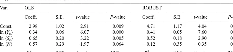
Table 2
Regression results for Solow’s growth model
Var. OLS ROBUST
Coeff. S.E. t-value P-value Coeff. S.E. t-value P-value
Const. 2.98 1.02 2.91 0.009 4.71 1.17 4.04 0.001
ln (Y )0 20.34 0.06 26.07 0.000 20.41 0.05 27.60 0.000
ln (S )k 0.65 0.20 3.22 0.005 0.52 0.18 2.90 0.011
ln (N ) 20.57 0.29 21.97 0.064 20.12 0.35 20.35 0.729
2 2
R 0.75 F-value 17.7 R 0.83 F-value 25.2
points, we retain them in the data set. Canada, Turkey, and New Zealand have standardized LTS residuals of 4.21, 26.14 and 23.16 and robust distances 7.25, 9.36, and 5.98 which together say that these are bad leverage points. We obtain different results reported in Table 2 when these countries are removed from the data set.
Elimination of these three countries has a large effect on the regression. As before, the fit is improved. Equally important, the population growth variable ln (N ), which is borderline significant in the original equation, appears insignificant in the robust regression.
5. Benderly and Zwick’s return data
Benderly and Zwick (1985) aim to explain the yearly return on USA common stocks by output growth and inflation, over the 1954–1981 period. Return on stocks is measured using the Ibbotson– Sinquefeld data base, output growth is proxied by the percentage change in real GNP, and inflation is measured by the deflator for personal consumption expenditures.
The regression equation concentrated on is:
Rt5b01b1Gt1b2 tI 1et (3)
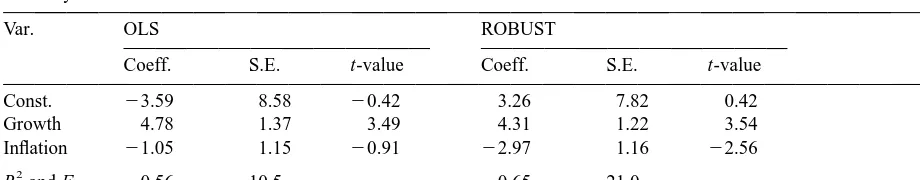
where R, G, and I stand for return on common stocks, output growth, and inflation, respectively. A standard OLS analysis reveals no outliers among these 28 years. However, a robust LTS analysis reveals that two of the observations have standardized residuals just outside of the 2.5 standard deviations tolerance band. In addition, these years have slightly high robust distances, hence they are mild leverage points. Indeed, the robust distances and the standardized LTS residuals are 3.65 and 2.60 for 1979, whereas they are 3.55 and 2.82 for 1980. OLS was run with and without these years, and the regression results for both OLS and ROBUST are displayed in Table 3.
Table 3
Benderly and Zwick’s data for return on common stocks
Var. OLS ROBUST
Coeff. S.E. t-value Coeff. S.E. t-value
Const. 23.59 8.58 20.42 3.26 7.82 0.42
Growth 4.78 1.37 3.49 4.31 1.22 3.54
Inflation 21.05 1.15 20.91 22.97 1.16 22.56
2
R and F 0.56 10.5 0.65 21.0
6. Concluding remarks
We have applied high breakdown robust regression techniques to several linear regression models found in the recent economic literature. In each case we observed that deleting a few outlying points has a big impact on the regression results. The fit often improves and the significance of the regressors changes, with implications for theory. The application of this technique is strongly recommended, even for simple regression, to avoid the misleading effects of bad leverage points.
The classification of data into groups of regular observations, bad leverage points, good leverage points, and vertical outliers, offers the researcher important diagnostic insight in the data. The good leverage points are very valuable, because they allow to obtain the regression fit with high precision. The bad leverage points pull the OLS regression fit in the wrong direction. The vertical outliers are also capable of strongly affecting the OLS regression fit: recall that the removal of just one such significant vertical outlier — belonging to Zambia — led to a drastic change of the regression results in De Long and Summers’ data set.
Although high breakdown robust regression techniques still take somewhat more computation time than plain OLS regression, their benefits more than outweigh the cost of applying them.
References
Belsley, D.A., Kuh, E., Welsch, R.E., 1980. Regression diagnostics: identifying influential data and sources of collinearity. In: Wiley Series in Probability and Mathematical Statistics. John Wiley, New York.
Benderly, J., Zwick, B., 1985. Inflation, real balances, output, and real stock returns. American Economic Review 75, 1115–1125.
De Long, J.B., Summers, L.H., 1991. Equipment investment and economic growth. Quarterly Journal of Economics 106, 445–501.
Knez, P.J., Ready, M.J., 1997. On the robustness of size and book-to-market in cross-sectional regressions. Journal of Finance 52, 1355–1382.
Krasker, W.S., Kuh, E., Welsch, R.E., 1983. Estimation for dirty data and flawed models. In: Griliches, Z., Intriligator, M.D. (Eds.). Handbook of Econometrics, Vol. 1. North-Holland, Amsterdam, pp. 651–698.
Mankiw, N.D., Romer, D., Weil, D., 1992. A contribution to the empirics of economic growth. Quarterly Journal of Economics 107, 407–437.
Rousseeuw, P.J., 1984. Least median of squares regression. Journal of the American Statistical Association 79, 871–880. Rousseeuw, P.J., Leroy, A.M., 1987. Robust regression and outlier detection. In: Wiley Series in Probability and
Mathematical Statistics. John Wiley, New York.
Rousseeuw, P.J., Van Driessen, K., 1998. Computing LTS regression for large data sets, Technical report. Universitaire Instelling Antwerpen (UIA), Belgium.
Rousseeuw, P.J., Van Driessen, K., 1999. A fast algorithm for the minimum covariance determinant estimator. Technometrics 41, 212–223.
Rousseeuw, P.J., Van Zomeren, B.C., 1990. Unmasking multivariate outliers and leverage points. Journal of the American Statistical Association 85, 633–639.
Rousseeuw, P.J., Wagner, J., 1994. Robust regression with a distributed intercept using least median of squares. Computational Statistics and Data Analysis 17, 65–76.
Yohai, V.J., 1987. High breakdown point and high efficiency robust estimates for regression. Annals of Statistics 15, 642–665.