AGGREGATE PLANNING TO MINIMIZE COST
OF PRODUCTION IN MANUFACTURING COMPANY
Enny Noegraheni
1;
Hasbi Nuradli
21,2Management Department, School of Business Management, Bina Nusantara University,
Jln. K.H. Syahdan No 9, Jakarta Barat, DKI Jakarta, 11480, Indonesia 1[email protected]; 2[email protected]
Received: 28th January 2016/ Revised: 10th May 2016/ Accepted: 13th May 2016
How to Cite: Noegraheni, E., & Nuradli, H. (2016). Aggregate Planning to Minimize Cost of Production in Manufacturing Company. Binus Business Review, 7(1), 39-45.
http://dx.doi.org/10.21512/bbr.v7i1.1448
ABSTRACT
The rapid growth of seafood industry has lead to fierce competition. PT Anela is one of the major players in its
industry. The company needs to develop a good strategy for competitive advantage in winning the competition. PT
Anela is one of the major players in the seafood industry. However, it has a limitation in production capacity. The objectives of this study were to calculate the forecast demand and to develop aggregate production planning for
PT Anela to meet demand with the lowest cost. The data were gathered through literature review and secondary data gathered directly from the company itself. The demand data from past three years was used to forecast demand using linear regression with seasonal index. Furthermore, all data were analyzed and used to design aggregate planning by using three strategies namely Chase, Level, and Mixed strategy which calculated by POM for Windows. The results of this study shows that the mixed strategy is the optimal strategy .
Keywords: aggregate planning, minimize cost, cost of production manufacturing company
INTRODUCTION
Effective and efficient production is necessary
to ensure the availability of products meet the needs of customers thus the implementation of the company’s operations are not having problems related to the planning of production which they have been made.
In the process of establishing an effective and efficient
production required more attention to contributor factors such as labor and machinery (the amount of labor and machinery), the production capacity of the machines used, cycle time, and scheduling shifts. When the production division already has reserves of
manpower and machinery to cope with the fluctuations
in demand for goods, the production can run on time, and the number of requests can be fulfilled.
However, when there is uncertainty about the amount of demand, usually a lot of manpower and machinery is unused (Nasution in Rahmadhani, Rahman & Tantrika, 2014). Food and beverage industry play an important role in economic growth
in Indonesia. Hartono (2015) reported the industry
minister Saleh Husin said in the first quarter of 2015, the
growth of national food and beverage industry reached 8.16%, the value has exceeded the targeted value of the Association of Indonesian Food and Beverages (GAPMMI) at the end of 2014 is 8%. The industry minister, Saleh Husin also said the contribution of the national food and beverage industry can be shown from the contribution value of their exports reach USD 456.6 million in January 2015, compared to the value of their exports in January 2014 USD 411.5 million.
Food and beverage market in Indonesia is growing positively inclined; attractive to foreign investors. National food and beverage industry proved to be one of the industries with the growth rate that is quite high in Indonesia. Rahman (2014) reported Association of Indonesian Food and Beverage (Gapmmi) said there are about 14 foreign investors from three countries, namely Japan, South Korea, and the United States, plans to enter the food and beverage industry in Indonesia. Higher foreign interest that will
Binus Business Review, 7(1), May 2016, 39-45 DOI: 10.21512/bbr.v7i1.1448
encourage investment in the industry is about 22 % next year to Rp 55 trillion from Rp 45 trillion said Adhi S Lukman, Chairman Gapmmi.
PT Anela is a seafood industry located in Jalan Raya Dendles km.82 Lamongan, East Java. For PT
Anela, fishball is the biggest source of profit. Fishball is a product made from fish mixed with other raw materials such as flour and condiments processed into meatballs and wrapped in packs of 10 kg per pack, the fish used include brass fish, knives fish, rambangan fish, custody fish and other fish from the fishermen. The positive growth of industry makes PT Anela faced
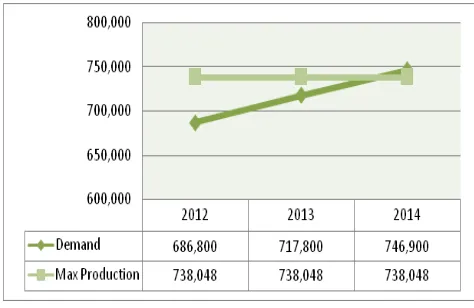
with increasingly high demand every year. According to Mr. Arifin Sulhan, President Director of PT Anela, sometimes the company cannot finish their production on time because the demand for fishball production in the last three years increase rapidly. Figure shows the demand and production of fishball for the past three
years.
Figure Demand and Production Source: PT Anela (2015)
There was increasing customer demand for 10 kg product from 2012 to 2014. The problem arose in 2014 when customer demand reached 746.9 thousand packs while the company has production capacity only 738.1 thousand packs, another problem was surplus
and shortage production.
Surplus production increases warehouse cost,
on the other hand, shortage production decrease the chance to meet customer needs. Production planning
and scheduling was the key issue to solve this problem.
PT Anela planned their production based on their past
experiences and estimation only (subjective planning), they also took overtime cost and took outside workers (sub-contracting) to meet specific production.
Food industry growth rapidly that the competition was a crucial issue. Future planning was an answer to win the competition; the planning
includes short, middle and long-term planning.
Pratanto (2012) in Rahmadhani, Rahman & Tantrika (2014) stated that the aggregate planning as a way to
equalize supply and demand number (for product or
services) with determining input time, transformation
time, output time and number of raw material properly.
Usually, the aggregate planning decisions made for the
production, staffing, inventory and back order level.
One of the goals of strategic planning to reduce the aggregate employment issues (overtime
and subcontracting), use of resources and equipment optimally and efficiently to minimize inventory number and to achieve minimal cost (Pratanto, 2012) in Rahmadhani, Rahman & Tantrika (2014).
The objective of production planning was to plan whole production planning and meet the demand by using production factors with minimal cost. The
purpose of this study is to predict the demand on PT
Anela in the period May 2015 - April 2016 and plan
aggregate planning to minimize production costs.
Forecasting (Heizer and Render, 2015) is the art
and science in predicting future events. Forecasting involves the retrieval of historical data (such as
sales last year) and projecting into the future with
mathematical models. According to Heizer and Render
(2015), there are two approaches to forecasting: (1) qualitative analysis and (2) quantitative analysis. Time Series Forecasting Method (Sugiyono, 2011)
is a quantitative forecasting method to determine the pattern of past data is collected in chronological order, called time series data. In this study, the method of Time Series used is Linear Regression. According
to Heizer and Render (2015), a linear regression is
a mathematical model of straight lines to describe
the functional relationship between the dependent
variable and independent. Time series forecasting,
linear regression formula suitable for use when the
data pattern is a trend. In forecasting, linear regression can be determined by the equation:
y = a + bx (1)
Where:
y = dependent variable
a = intercept (value of Y when X = 0)
b = slope of regression line x = independent variable
Heizer and Render (2015) stated that the
aggregate planning is an approach to determine the quantity and timing of production in the medium
term (usually) 3 to 18 months. Aggregate planning
problem can be solved by considering a variety of available options. Planning decisions are planning for production labor, materials, machinery, and other
equipment as well as the capital required to produce
goods at a certain period in the future in accordance
with the estimated or predicted Bedwoth in Cahyono (2007). Aggregate planning strategy by Heizer and Render (2015) consists of five first-choice called
capacity options because this option is not trying to
change requests, but to absorb fluctuations in demand. The last three choices are the choice of request which
Capacity options also known as a pure strategy
is an option that seeks not to change a demand but to
absorb fluctuations of demand by converting available capacity. Capacity selection consists of five options, namely: (1) changing the number of workers (hire and fire). One way to meet the demand by hiring or firing workers depend on production levels. (2)
Varying levels of production through overtime or idle
time. A number of worker s can be kept constant by changing working hours. (3) Sub-contract: a company
can obtain temporary capacity by subcontracting their
worker during high demand periods. (4) Using time worker: especially in the service sector, a part-time worker can fill the needs of part-part-time unskilled
labor. This is a common practice in restaurants, retail
stores, and supermarkets business. (5) Change the
regular inventory: manager improves inventory levels
during low period of demand to meet the high demand
in the future.
Options demand are consisted of three basic
demands. First, influencing the demand; when low
demand session, company could increase the demand through advertising, promotion, personal sales and discounts price. Second, amount overdue orders during
high demand period; amount overdue orders is an order
of goods or services received by the company but can
not afford (intentional or accidental) to be met at this
time. Third, mix the products and services against seasonal trends. An active and smooth technique that
is widely used by manufacturers by developing the
product mix of the goods against seasonal trends.
According to Heizer and Render (2015), the
aggregate planning can be done by making a choice
of three strategies; Chase Strategy, Level Scheduling
Strategy and Mixed Strategy. Here’s an explanation of
each strategy: (1) Chase Strategy, a planning strategy
that is set a number of demand equal to the number of forecast demand production (production adjusted
to demand). This strategy tries to achieve the level
of output for each period meets the demand forecast
for the period; (2) Level Scheduling Strategy, is the aggregate plan in which the rate of production remains the same from period to period (constant output).
Scheduling levels maintain output levels, production levels, or levels of employment constant in the
planning horizon; (3) Mixed Strategy, this strategy
involves changing more than one variable that can
be controlled (controllable decision variable). Some
combination of changing variables can be controlled to produce a planning strategy that best aggregate.
According to Simamora and Natalia (2014), a Mixed Strategy is a composite strategy between the
Chase Strategy and Level Strategy. This strategy takes
benefit from advantages and disadvantages of Chase
Strategy and Level Strategy to reduce the negative impact of pure alternative strategy. Input aggregate
planning according to Sukendar and Kristomi (2008),
is the necessary information to make an aggregate
planning effective, namely: (1) the resources available
throughout the period of the plan of production must
be known, (2) data requests coming from forecasting
and order later translated into the level of production,
(3) incorporating the company’s policy with respect
to the aggregate planning, for example, changes in the level of employment, and the determination of resource requirements.
While aggregate output planning, according
to Sukendar and Kristomi (2008), is the aggregate
planning process usually a production schedule for classifying products based on the “family”. For instance, for car manufacturers, the output provides
information on how cars should be produced, but not on how many cars are branded A, series B, and C. So
the form of the overall amount of output produced for each period rather than for each type.
Nasution and Prasetyawan in Octavianti et al.,
(2013) suggested the costs involved in planning the aggregate are: (1) Hiring Cost (additional cost for labor cost) is the costs for advertising, selection and training. (2) Firing Cost (cost for dismissal labor) in the form of severance pay for employees who are
laid off, declining morale and productivity employees
who are still working, and the pressure of a social nature. (3) Overtime Cost and Approaches Cost. The additional cost of overtime is usually 150% of the cost of regular work, whereas when the surplus of labor
can not be allocated effectively, then the company
considered bearing the idle cost. (4) Inventory Cost and Backorder Cost. The Inventory Cost in the form
of retention of capital costs, taxes, insurance, material
damage, and the cost of renting warehouse. The Backorder Cost is calculated based on how many items requested were not available. (5) Subcontract Cost is the cost paid by the company when demand exceeds
the regular capacity so that the excess demand can not be handled and subcontracted to other companies.
Aggregate planning method, according to
Heizer and Render (2015); Radwan and Aarabi (2011),
are several techniques that can be used to operational manager develop an aggregate planning. First, graphical techniques is a very popular technique because it is easy
to be understood and used. Basically, this plan uses
several variables so planners can compare projected
demand with current capacity. This approach is a trial
approach and does not assure an optimal production plan, but only requires limited computation. Here are
five stages in the graphical method. First, determine
the demand in each period. Second, determine the capacity for regular time, overtime, subcontracting in each period. Third, calculate the cost of labor,
cost of hire and fire workers, and inventory storage
costs. Fourth, consider a company policy that can be applied to labor or inventory levels. Fifth, develop alternative plans and examine the total costs. Second, mathematical approach, the transportation method of linear programming, its is one of the mathematical approach generates an optimal plan to minimize
costs. Transportation method also flexible because it
can specify the production of regular and overtime in each period, the number of units to be subcontracted, additional shifts and supplies brought from one period
METHODS
The research method was a systematic series
of stages that must be set before the resolution of the problem being discussed. Type a descriptive research, i.e., research that its main characteristic is to provide an objective explanation, comparison, and evaluation as a decision for the authorities.
Data were collected by survey techniques (field research) which aims to search for a problem that occurs in the company. The way of collecting the data are consisted of three ways. Firstly, observation is
namely the collection of data by conducting a direct observation of scheduling production at PT Anela.
Secondly, interviews, by performing the question and answer session and discussion to obtain information
about the timing and the problems experienced. The third method is documentation, to see and use reports and records that exist in the company. The second
method is literature study (library research) which aims
to solve problem that has been formulated based on
the theory of previous research and other information. Analyzing problems that occur in the PT Anela
uses several methods. The first method is linear regression with season index for forecasting demand.
The second method consists of the three alternative
strategies (chase, level and mixed) for aggregate
planning. In analyzing the problem of production
capacity in the period that has been specified in the
PT Anela, optimizing all the resources of the company to minimize any costs is done by adjusting production value based on the requests number.
The sales data for the last three years (May
2012 - April 2015) are to determine the predictive forecasting demand for the next year (May 2015 - April 2016). According to Sugiyono (2011), linear
regression analysis is a mathematical model of straight
lines to describe the functional relationship between
the dependent variables and the independent variable.
The dependent variable wanting forecast to remain the
same, namely y and independent variable is x by the
following equation: y = a + bx.
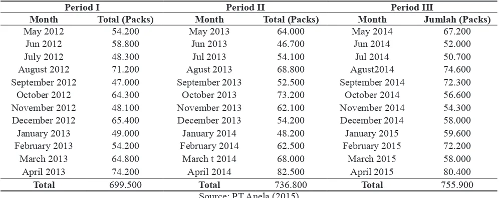
Table 1 Annual Sales
Period I Period II Period III
Month Total (Packs) Month Total (Packs) Month Jumlah (Packs)
May 2012 54.200 May 2013 64.000 May 2014 67.200
Jun 2012 58.800 Jun 2013 46.700 Jun 2014 52.000
July 2012 48.300 Jul 2013 54.100 Jul 2014 50.700
August 2012 71.200 Agust 2013 68.800 Agust2014 74.600 September 2012 47.000 September 2013 52.500 September 2014 72.300 October 2012 64.300 October 2013 73.200 October 2014 56.600 November 2012 48.100 November 2013 62.100 November 2014 54.300 December 2012 65.400 December 2013 54.200 December 2014 58.000 January 2013 49.000 January 2014 48.200 January 2015 59.600 February 2013 54.200 February 2014 62.500 February 2015 72.200 March 2013 64.800 March t 2014 68.000 March 2015 58.000 April 2013 74.200 April 2014 82.500 April 2015 80.400
Total 699.500 Total 736.800 Total 755.900
Source: PT Anela (2015)
Table 2 Solution
No. Strategy Cost Method
1. Chase Strategy • Production cost (regular)
• Production cost (overtime)
• Sub-contracted cost
• Inventory shortage cost
• Chase current demand POM for Windows
2. Level Strategy • Production cost (regular)
• Production cost (overtime)
• Sub-contracted cost
• Inventory maintenance cost
• Inventory shortage cost
• Average gross demand POM for Windows
3. Mixed Strategy • Production cost (regular)
• Production cost (overtime)
• Sub-contracted cost
• Inventory maintenance cost
• The transportation method of linear programming POM for Windows
Some data needed to calculate the aggregate
planning are (1) the production capacity , the capacity of which owned by the company’s production process.
The production capacity consists of regular production capacity, overtime capacity, speed of production, and
subcontracting policies set by the company; (2) The cost of production, data which support an important
role in the calculation of aggregate planning is the regular production costs, the production cost of overtime and subcontracting costs, handling costs and the cost of inventory shortages. In analyzing the capacity problems that occur in the PT Anela, researchers optimize all the company’s resources to minimize all costs incurred to meet customer demand
by using POM software for Windows.
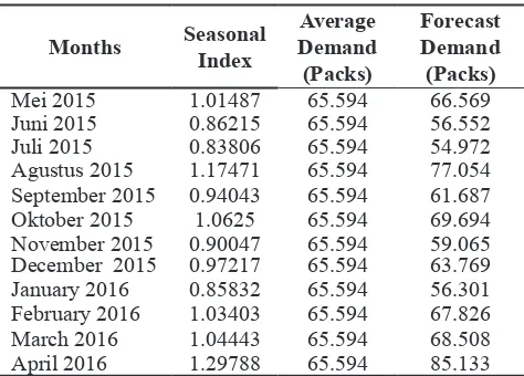
RESULTS AND DISCUSSIONS
The demand forecast in May 2015 - April 2016, using fishball demand data for three previous years, i.e., from May 2012 - April 2015 can be viewed in Mei 2015 1.01487 65.594 66.569 Juni 2015 0.86215 65.594 56.552 Juli 2015 0.83806 65.594 54.972 Agustus 2015 1.17471 65.594 77.054 September 2015 0.94043 65.594 61.687 Oktober 2015 1.0625 65.594 69.694 November 2015 0.90047 65.594 59.065 December 2015 0.97217 65.594 63.769 January 2016 0.85832 65.594 56.301 February 2016 1.03403 65.594 67.826 March 2016 1.04443 65.594 68.508 April 2016 1.29788 65.594 85.133
Source: Research Result (2015)
The company’s ability to produce is viewable through the data capacity: (1) In regular production, the company can produce 2,480 packs with the number of workers needed in the production of fishball is 200 people with eighth working hours per day. (2) Fishball of production per hour time is 8 hours per day (2480 packs/200 workers) is 0,645 hours. (3) Companies limit overtime hours i.e. ten days a month, two
hours per day. In an hour the company can produce
310 packs. So overtime production capacity is 6,200 packs per month. (4) The company has a policy to limit subcontracting maximum of 7,000 packs per month when the company unable meet the demand. The restriction was made because of the high cost of
subcontracting.
First, the cost of regular production (regular time
cost) per wrappings is obtained by adding up the cost of raw materials, labor costs, the cost of machinery
and buildings and other expenses such as the cost of
electricity and water. The data obtained from PT Anela listed as follows: (1) based on the company estimates the average cost of raw materials for the manufacture of fishball every day at Rp. 90,000,000.00. So the cost of production per pack is Rp. 90,000,000.00/2480 packs per day, Rp. 36290.00 per pack; (2) worker wage set by the Company is Rp. 8000.00 per hour. Time to produce a pack of fishball is 0,645 hours. So labor costs per pack Rp. 8000.00 x 0,645, Rp. 5160.00; (3)
the cost of machinery and buildings is the cost of the use of machinery and buildings set companies per year
is Rp. 125,000,000.00. While the number of working days in the planning period is 298 days. So the cost per pack is Rp. 125,000,000.00/298x2480 Rp. 169.13; (4) other charges, namely electricity and water per month is Rp. 4.500.000, and Rp. 1.500.000,00. The average working day in a month is 25 days. So the cost of electricity and water per pack is Rp 6.000.000,00/ (25x2480) is Rp. 96.77.
Table 4 Cost per Packs (Fish ball)
Raw material cost Rp 36.290,00 Worker cost Rp 5.160,00 Machinery and building cost Rp 169,13 Other cost Rp 96,77
Total Rp 41.715,90
Source: Research Result (2015)
Second, overtime cost at PT Anela is Rp
44295.90 by totaling the cost of labor and a half times the regular fee of Rp. 7,740 and other costs the same as regular costs, such as raw material costs, costs
of machinery and buildings and other costs such as
electricity and water; Third, the cost of subcontracting is Rp 47000.00 per pack. This price is determined
by the company that sells its products to PT Anela. Subcontracting costs have higher costs than the
production itself;
Fourth, the inventory cost which consists of the accumulated cost of the warehouse with refrigeration machine with a capacity of 600 tons, warehouse workers, and the use of electricity at a predetermined company is Rp 80.00 per pack. Fifth, shortage cost
is the cost incurred by the company if the request
cannot be met by the company, Rp 20,000.00 per pack
obtained from the company’s policy. Sixth, the cost of
excess production (increase of unit cost). In this case,
company policy does not take into account such costs,
so the cost is £ 0.00. Seventh, the decrease unit cost.
In this case company policy does not take into account
such costs, so the cost is £ 0.00.
Based on historical data, the data has a trend. According to Heizer and Render (2015), the trend is a gradual movement of data either upwards or downwards over the years, so the demand forecast one year ahead using linear regression approach. The first
determine the next year request. Figures in the index numbers on the season describe future demand. After
finding the seasonal index which determines the total demand of May 2015 - April 2016, linear regression approach was used. Mei 2015 1.01487 65.594 66.569 Juni 2015 0.86215 65.594 56.552 Juli 2015 0.83806 65.594 54.972 Agustus 2015 1.17471 65.594 77.054 September 2015 0.94043 65.594 61.687 Oktober 2015 1.0625 65.594 69.694 November 2015 0.90047 65.594 59.065 December 2015 0.97217 65.594 63.769 January 2016 0.85832 65.594 56.301 February 2016 1.03403 65.594 67.826 March2016 1.04443 65.594 68.508 April 2016 1.29788 65.594 85.133
Source: Research Result (2015)
The first alternative is a chase strategy, to achieve the level of output in accordance with the demand
forecast for the period. The second alternative is a strategy level to achieve a stable output level of each
month. The third alternative is a mixed strategy, which is a combination of the two previous alternatives. In this case, researcher used POM for Windows.
Chase Strategy is a strategy to produce a
number of products in accordance with the demand
forecast for that month. Companies must produce the
right amount of product in accordance with the request
through the regular production, overtime production and also this sub-contracted. This strategy matches production levels and the number of the requests in the period of the strategy. Inventory maintenance cost does not determine in this strategy.
Level Strategy is a strategy that equalize the level of production in each month of a planning period.
The company must reach a level of production with
the regular production, overtime and subcontracting.
In this strategy subcontracting costs and lower cost
inventory shortage, but has cost storage handlers in production activities.
Mixed Strategy aims to produce output in
accordance with a production capacity of regular
time, subcontracting and overtime optimally so as to meet the needs of every month. This strategy seeks to
avoid shortage of inventory when it occurs can lead
customer loses and dissatisfaction. Mixed Strategy
calculated using the method of transportation to find
the optimal solution.
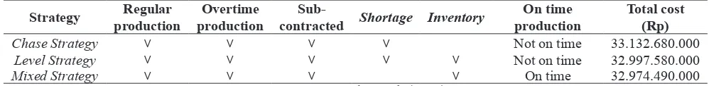
Chase Strategy ˅ ˅ ˅ ˅ Not on time 33.132.680.000
Level Strategy ˅ ˅ ˅ ˅ ˅ Not on time 32.997.580.000
Mixed Strategy ˅ ˅ ˅ ˅ On time 32.974.490.000
Source: Research Result (2015) Table 6 Comparison of Three Strategies
Here is a comparison of the three strategies. First, Chase Strategy using regular production, overtime and subcontracting production to meet demand, but from the results obtained contained high levels of inventory shortage because this strategy has not been able to meet demand on time. Chase Strategy manufacture products according to the demand at that time so it does not use any inventory handling. Second, level strategy using regular production, overtime, and subcontracting production to meet demand, but there is still a shortage of supply to meet demand and the level of strategy are handling the inventory to meet the demand in the next month.
Finally, Mixed Strategy combines both strategies. Mixed Strategy using regular production,
overtime, and subcontracting production. In this strategy, there is no shortage of supply so that demand can be met in the planning period and there isa handling
charge of inventory. By using a Mixed Strategy, the company was able to meet the demand on time at the lowest cost. Most firms find it advantageous to
utilize a combination of the Level Strategy and Chase
Strategy. A combination strategy (called as Hybrid or
Mixed Strategy) can be found to meet organizational goals and policies and achieve lower costs than either
of the pure strategies used independently, according
to Chinguwa, Madanhire, and Musoma (2013). Based on Radwan and Aarabi (2011), Mixed Strategy is a
combination of Chase Strategy and Level Strategy. It is often used to evaluate large-scale enterprise business needs. Chase Strategy aligns production to
meet the demand with minimum inventory level. Level Strategy plans in which the aggregate production
level remains the same for a period of time (constant
output). Scheduling levels maintain output levels,
production levels, or constant employment levels in the planning horizon.
CONCLUSIONS
There are several conclusions that can be
which has been processed using linear regression with the seasonal index for three years back, showed a
trend increase every year. A mixed Strategy is the best alternative for PT Anela. Some suggestions that can be concluded from the research is forecasting should be done to anticipate number of demand and tends to
increase and for the planning period between May 2015 - April 2016. Also, the best strategy is mixed
solution by using the transportation method of linear programming.
REFERENCES
Cahyono, D. D. (2007). Perencanaan Produksi Disagregasi Dengan Pendekatan Reguler Knapsack Method Pada Produk Mini Boom ZX 25 YYZX22B dan Mini Boom ZX 30 YYZX30B. Retrieved from http://library. gunadarma.ac.id.
Chinguwa, S., Madanhire, I., & Musoma, T. (2013). A Decision Framework based on Aggregate Production Planning Strategies in a Multi Product Factory: A Furniture Industry Case Study. International Journal of Science and Research (IJSR), India Online, 2(2), 370-383.
Hartono (Ed). (2015, 26 May). Triwulan I tahun2015, Industri Makanan dan Minuman Capai 8,16%. Retrieved August 15th, 2015 from http://www. kemenperin.go.id/
Heizer, J. H. & Render, B. (2015). Manajemen Operasi: Manajemen Keberlangsungan dan Rantai Pasokan (11th ed.). Jakarta: Salemba Empat.
Octavianti, I. A., Setyanto, N. W., & Tantrika, C. F. M. (2013). Perencanaan Produksi Agregat Produk Tembakau Rajang P01 dan P02 di PT. X. Jurnal Rekayasa dan Manajemen Sistem Industri, 1(2), 264-274.
Radwan, A., & Aarabi, M. (2011). Study of Implementing Zachman Framework for Modeling Information Systems for Manufacturing Enterprises Aggregate Planning. Proceedings of the 2011 International Conference on Industrial Engineering and Operations Management, Kuala Lumpur, Malaysia. Rahmadhani, A., Rahman, A., & Tantrika, C. F. M. (2014).
Perencanaan Agregat Chase Strategy dengan Analisis Kebutuhan Operator dan Sesuai Fluktuasi Permintaan Rokok (Studi Kasus: PR. Adi Bungsu, Malang). Jurnal Rekayasa dan Manajemen Sistem Industri, 2(6), 1192-1202.
Rahman, D. (Ed). (2014, 23 December). Investasi Sektor Makanan Topang Pertumbuhan Industri pada 2015. Retrieved March 22th, 2015 from http://www.ift. co.id/
Simamora, B. H., & Natalia, D. (2014). Aggregate Planning for Minimizing Costs: A Case Study of PT XYZ in Indonesia. International Business Management, 8(6), 353-35.
Sugiyono. (2011). Metode Penelitian Kuantitatif, Kualitatif dan R&D. Bandung: Alfabeta.