•Buildanopticalcharacterrecognition(OCR)systemfromscratch •Codeaspamfilterthatlearnsbyexample
•UseF#’spowerfultypeproviderstointerfacewithexternalresources (inthiscase,dataanalysistoolsfromtheRprogramminglanguage) •Transformyourdataintoinformativefeatures,andusethemtomake •Findpatternsindatawhenyoudon’tknowwhatyou’relookingfor •Predictnumericalvaluesusingregressionmodels
For your convenience Apress has placed some of the front
matter material after the index. Please use the Bookmarks
Contents at a Glance
About the Author ...
xiii
About the Technical Reviewer ...
xv
Acknowledgments ...
xvii
Introduction ...
.xix
■
Chapter 1: 256 Shades of Gray ...
1
■
Chapter 2: Spam or Ham? ...
33
■
Chapter 3: The Joy of Type Providers ...
67
■
Chapter 4: Of Bikes and Men ...
93
■
Chapter 5: You Are Not a Unique Snowflake ...
131
■
Chapter 6: Trees and Forests ...
179
■
Chapter 7: A Strange Game ...
211
■
Chapter 8: Digits, Revisited ...
239
■
Chapter 9: Conclusion ...
267
Introduction
If you are holding this book, I have to assume that you are a .NET developer interested in machine learning. You are probably comfortable with writing applications in C#, most likely line-of-business applications. Maybe you have encountered F# before, maybe not. And you are very probably curious about machine learning. The topic is getting more press every day, as it has a strong connection to software engineering, but it also uses unfamiliar methods and seemingly abstract mathematical concepts. In short, machine learning looks like an interesting topic, and a useful skill to learn, but it’s difficult to figure out where to start.
This book is intended as an introduction to machine learning for developers. My main goal in writing it was to make the topic accessible to a reader who is comfortable writing code, and is not a mathematician. A taste for mathematics certainly doesn’t hurt, but this book is about learning some of the core concepts through code by using practical examples that illustrate how and why things work.
But first, what is machine learning? Machine learning is the art of writing computer programs that get better at performing a task as more data becomes available, without requiring you, the developer, to change the code.
This is a fairly broad definition, which reflects the fact that machine learning applies to a very broad range of domains. However, some specific aspects of that definition are worth pointing out more closely. Machine learning is about writing programs—code that runs in production and performs a task—which makes it different from statistics, for instance. Machine learning is a cross-disciplinary area, and is a topic relevant to both the mathematically-inclined researcher and the software engineer.
The other interesting piece in that definition is data. Machine learning is about solving practical problems using the data you have available. Working with data is a key part of machine learning; understanding your data and learning how to extract useful information from it are quite often more important than the specific algorithm you will use. For that reason, we will approach machine learning starting with data. Each chapter will begin with a real dataset, with all its real-world imperfections and surprises, and a specific problem we want to address. And, starting from there, we will build a solution to the problem from the ground up, introducing ideas as we need them, in context. As we do so, we will create a foundation that will help you understand how different ideas work together, and will make it easy later on to productively use libraries or frameworks, if you need them.
Our exploration will start in the familiar grounds of C# and Visual Studio, but as we progress we will introduce F#, a .NET language that is particularly suited for machine learning problems. Just like machine learning, programming in a functional style can be intimidating at first. However, once you get the hang of it, F# is both simple and extremely productive. If you are a complete F# beginner, this book will walk you through what you need to know about the language, and you will learn how to use it productively on real-world, interesting problems.
256 Shades of Gray
Building a Program to Automatically Recognize
Images of Numbers
If you were to create a list of current hot topics in technology, machine learning would certainly be somewhere among the top spots. And yet, while the term shows up everywhere, what it means exactly is often shrouded in confusion. Is it the same thing as “big data,” or perhaps “data science”? How is it different from statistics? On the surface, machine learning might appear to be an exotic and intimidating specialty that uses fancy mathematics and algorithms, with little in common with the daily activities of a software engineer.
In this chapter, and in the rest of this book, my goal will be to demystify machine learning by working through real-world projects together. We will solve problems step by step, primarily writing code from the ground up. By taking this approach, we will be able to understand the nuts and bolts of how things work, illustrating along the way core ideas and methods that are broadly applicable, and giving you a solid foundation on which to build specialized libraries later on. In our first chapter, we will dive right in with a classic problem—recognizing hand-written digits—doing a couple of things along the way:
• Establish a methodology applicable across most machine learning problems.
Developing a machine learning model is subtly different from writing standard line-of-business applications, and it comes with specific challenges. At the end of this chapter, you will understand the notion of cross-validation, why it matters, and how to use it.
• Get you to understand how to “think machine learning” and how to look at ML
problems. We will discuss ideas like similarity and distance, which are central to most algorithms. We will also show that while mathematics is an important ingredient of machine learning, that aspect tends to be over-emphasized, and some of the core ideas are actually fairly simple. We will start with a rather straightforward algorithm and see that it actually works pretty well!
• Know how to approach the problem in C# and F#. We’ll begin with implementing the
solution in C# and then present the equivalent solution in F#, a .NET language that is uniquely suited for machine learning and data science.
What Is Machine Learning?
But first, what is machine learning? At its core, machine learning is writing programs that learn how to perform a task from experience, without being explicitly programmed to do so. This is still a fuzzy definition, and begs the question: How do you define learning, exactly? A somewhat dry definition is the following: A program is learning if, as it is given more data points, it becomes automatically better at performing a given task. Another way to look at it is by flipping around the definition: If you keep doing the same thing over and over again, regardless of the results you observe, you are certainly not learning.
This definition summarizes fairly well what “doing machine learning” is about. Your goal is to write a program that will perform some task automatically. The program should be able to learn from experience, either in the form of a pre-existing dataset of past observations, or in the form of data accumulated by the program itself as it performs its job (what’s known as “online learning”). As more data becomes available, the program should become better at the task without your having to modify the code of the program itself.
Your job in writing such a program involves a couple of ingredients. First, your program will need data it can learn from. A significant part of machine learning revolves around gathering and preparing data to be in a form your program will be able to use. This process of reorganizing raw data into a format that better represents the problem domain and that can be understood by your program is called feature extraction.
Then, your program needs to be able to understand how well it is performing its task, so that it can adjust and learn from experience. Thus, it is crucial to define a measure that properly captures what it means to “do the task” well or badly.
Finally, machine learning requires some patience, an inquisitive mind, and a lot of creativity! You will need to pick an algorithm, feed it data to train a predictive model, validate how well the model performs, and potentially refine and iterate, maybe by defining new features, or maybe by picking a new algorithm. This cycle—learning from training data, evaluating from validation data, and refining—is at the heart of the machine learning process. This is the scientific method in action: You are trying to identify a model that adequately predicts the world by formulating hypotheses and conducting a series of validation experiments to decide how to move forward.
Before we dive into our first problem, two quick comments. First, this might sound like a broad description, and it is. Machine learning applies to a large spectrum of problems, ranging all the way from detecting spam email and self-driving cars to recommending movies you might enjoy, automatic translation, or using medical data to help with diagnostics. While each domain has its specificities and needs to be well understood in order to successfully apply machine learning techniques, the principles and methods remain largely the same.
Then, note how our machine learning definition explicitly mentions “writing programs.” Unlike with statistics, which is mostly concerned with validating whether or not a model is correct, the end goal of machine learning is to create a program that runs in production. As such, it makes it a very interesting area to work in, first because it is by nature cross-disciplinary (it is difficult to be an expert in both statistical methods and software engineering), and then because it opens up a very exciting new field for software engineers.
Now that we have a basic definition in place, let’s dive into our first problem.
A Classic Machine Learning Problem: Classifying Images
and digits written by various people, computers have a hard time dealing with that task. This is the reason CAPTCHAs are such a simple and effective way to figure out whether someone is an actual human being or a bot. The human brain has this amazing ability to recognize letters and digits, even when they are heavily distorted.
FUN FACT: CAPTCHA AND RECAPTCHA
CAPTCHA (“Completely Automated Public
Turing test
to tell Computers and Humans Apart”) is a
mechanism devised to filter out computer bots from humans. To make sure a user is an actual
human being, CAPTCHA displays a piece of text purposefully obfuscated to make automatic computer
recognition difficult. In an intriguing twist, the idea has been extended with reCAPTCHA. reCAPTCHA
displays two images instead of just one: one of them is used to filter out bots, while the other is an
actual digitized piece of text (see Figure
1-1
). Every time a human logs in that way, he also helps digitize
archive documents, such as back issues of the
New York Times
, one word at a time.
Figure 1-1. A reCAPTCHA example
Our Challenge: Build a Digit Recognizer
The problem we will tackle is known as the “Digit Recognizer,” and it is directly borrowed from a Kaggle.com machine learning competition. You can find all the information about it here: http://www.kaggle.com/c/ digit-recognizer.
Here is the challenge: What we have is a dataset of 50,000 images. Each image is a single digit, written down by a human, and scanned in 28 ´ 28 pixels resolution, encoded in grayscale, with each pixel taking one of 256 possible shades of gray, from full white to full black. For each scan, we also know the correct answer, that is, what number the human wrote down. This dataset is known as the training set. Our goal now is to write a program that will learn from the training set and use that information to make predictions for images it has never seen before: is it a zero, a one, and so on.
So, how could we approach this problem? Let’s start with a different question first. Imagine that we have just two images, a zero and a one (see Figure 1-2):
Suppose now that I gave you the image in Figure 1-3 and asked you the following question: Which of the two images displayed in Figure 1-2 is it most similar to?
As a human, I suspect you found the question trivial and answered “obviously, the first one.” For that matter, I suspect that a two-year old would also find this a fairly simple game. The real question is, how could you translate into code the magic that your brain performed?
One way to approach the problem is to rephrase the question by flipping it around: The most similar image is the one that is the least different. In that frame, you could start playing “spot the differences,” comparing the images pixel by pixel. The images in Figure 1-4 show a “heat map” of the differences: The more two pixels differ, the darker the color is.
Figure 1-2. Sample digitized 0 and 1
In our example, this approach seems to be working quite well; the second image, which is “very different,” has a large black area in the middle, while the first one, which plots the differences between two zeroes, is mostly white, with some thin dark areas.
Distance Functions in Machine Learning
We could now summarize how different two images are with a single number, by summing up the differences across pixels. Doing this gives us a small number for similar images, and a large one for
dissimilar ones. What we managed to define here is a “distance” between images, describing how close they are. Two images that are absolutely identical have a distance of zero, and the more the pixels differ, the larger the distance will be. On the one hand, we know that a distance of zero means a perfect match, and is the best we can hope for. On the other hand, our similarity measure has limitations. As an example, if you took one image and simply cloned it, but shifted it (for instance) by one pixel to the left, their distance pixel-by-pixel might end up being quite large, even though the images are essentially the same.
The notion of distance is quite important in machine learning, and appears in most models in one form or another. A distance function is how you translate what you are trying to achieve into a form a machine can work with. By reducing something complex, like two images, into a single number, you make it possible for an algorithm to take action—in this case, deciding whether two images are similar. At the same time, by reducing complexity to a single number, you incur the risk that some subtleties will be “lost in translation,” as was the case with our shifted images scenario.
Distance functions also often appear in machine learning under another name: cost functions. They are essentially the same thing, but look at the problem from a different angle. For instance, if we are trying to predict a number, our prediction error—that is, how far our prediction is from the actual number—is a distance. However, an equivalent way to describe this is in terms of cost: a larger error is “costly,” and improving the model translates to reducing its cost.
Start with Something Simple
But for the moment, let’s go ahead and happily ignore that problem, and follow a method that has worked wonders for me, both in writing software and developing predictive models—what is the easiest thing that could possibly work? Start simple first, and see what happens. If it works great, you won’t have to build anything complicated, and you will be done faster. If it doesn’t work, then you have spent very little time building a simple proof-of-concept, and usually learned a lot about the problem space in the process. Either way, this is a win.
So for now, let’s refrain from over-thinking and over-engineering; our goal is to implement the least complicated approach that we think could possibly work, and refine later. One thing we could do is the following: When we have to identify what number an image represents, we could search for the most similar (or least different) image in our known library of 50,000 training examples, and predict what that image says. If it looks like a five, surely, it must be a five!
The outline of our algorithm will be the following. Given a 28 ´ 28 pixels image that we will try to recognize (the “Unknown”), and our 50,000 training examples (28 ´ 28 pixels images and a label), we will:
• compute the total difference between Unknown and each training example; • find the training example with the smallest difference (the “Closest”); and • predict that “Unknown” is the same as “Closest.”
Let’s get cracking!
Our First Model, C# Version
To get warmed up, let’s begin with a C# implementation, which should be familiar territory, and create a C# console application in Visual Studio. I called my solution DigitsRecognizer, and the C# console application
CSharp— feel free to be more creative than I was!
Dataset Organization
The first thing we need is obviously data. Let’s download the dataset trainingsample.csv from
http://1drv.ms/1sDThtz and save it somewhere on your machine. While we are at it, there is a second file in the same location, validationsample.csv, that we will be using a bit later on, but let’s grab it now and be done with it. The file is in CSV format (Comma-Separated Values), and its structure is displayed in Figure 1-5. The first row is a header, and each row afterward represents an individual image. The first column (“label”), indicates what number the image represents, and the 784 columns that follow (“pixel0”, “pixel1”, ...) represent each pixel of the original image, encoded in grayscale, from 0 to 255 (a 0 represents pure black, 255 pure white, and anything in between is a level of gray).
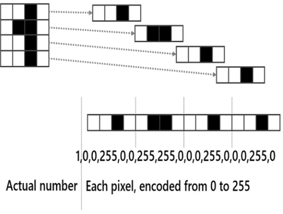
For instance, the first row of data here represents number 1, and if we wanted to reconstruct the actual image from the row data, we would split the row into 28 “slices,” each of them representing one line of the image: pixel0, pixel1, ..., pixel 27 encode the first line of the image, pixel28, pixel29, ..., pixel55 the second, and so on and so forth. That’s how we end up with 785 columns total: one for the label, and 28 lines ´ 28 columns = 784 pixels. Figure 1-6 describes the encoding mechanism on a simplified 4 ´ 4 pixels image: The actual image is a 1 (the first column), followed by 16 columns representing each pixel’s shade of gray.
Figure 1-6. Simplified encoding of an image into a CSV row
■
Note
If you look carefully, you will notice that the file trainingsample.csv contains only 5,000 lines, instead
of the 50,000 I mentioned earlier. I created this smaller file for convenience, keeping only the top part of the
original. 50,000 lines is not a huge number, but it is large enough to unpleasantly slow down our progress, and
working on a larger dataset at this point doesn’t add much value.
Reading the Data
As a first step, we need to read the data from the CSV file into a collection of observations. Let’s go to our solution and add a class in the CSharp console project in which to store our observations:
Listing 1-1. Storing data in an Observation class
public class Observation {
public Observation(string label, int[] pixels) {
this.Label = label; this.Pixels = pixels; }
public string Label { get; private set; } public int[] Pixels { get; private set; } }
Next, let’s add a DataReader class with which to read observations from our data file. We really have two distinct tasks to perform here: extracting each relevant line from a text file, and converting each line into our observation type. Let’s separate that into two methods:
Listing 1-2. Reading from file with a DataReader class
public class DataReader {
private static Observation ObservationFactory(string data) {
var commaSeparated = data.Split(','); var label = commaSeparated[0]; var pixels =
commaSeparated .Skip(1)
.Select(x => Convert.ToInt32(x)) .ToArray();
return new Observation(label, pixels); }
public static Observation[] ReadObservations(string dataPath) {
var data =
File.ReadAllLines(dataPath) .Skip(1)
.Select(ObservationFactory) .ToArray();
return data; }
Note how our code here is mainly LINQ expressions! Expression-oriented code, like LINQ (or, as you’ll see later, F#), helps you write very clear code that conveys intent in a straightforward manner, typically much more so than procedural code does. It reads pretty much like English: “read all the lines, skip the headers, split each line around the commas, parse as integers, and give me new observations.” This is how I would describe what I was trying to do, if I were talking to a colleague, and that intention is very clearly reflected in the code. It also fits particularly well with data manipulation tasks, as it gives a natural way to describe data transformation workflows, which are the bread and butter of machine learning. After all, this is what LINQ was designed for—“Language Integrated Queries!”
We have data, a reader, and a structure in which to store them—let’s put that together in our console app and try this out, replacing PATH-ON-YOUR-MACHINE in trainingPath with the path to the actual data file on your local machine:
Listing 1-3. Console application
class Program {
static void Main(string[] args) {
var trainingPath = @"PATH-ON-YOUR-MACHINE\trainingsample.csv"; var training = DataReader.ReadObservations(trainingPath);
Console.ReadLine(); }
}
If you place a breakpoint at the end of this code block, and then run it in debug mode, you should see that training is an array containing 5,000 observations. Good—everything appears to be working.
Our next task is to write a Classifier, which, when passed an Image, will compare it to each
Observation in the dataset, find the most similar one, and return its label. To do that, we need two elements: a Distance and a Classifier.
Computing Distance between Images
Let’s start with the distance. What we want is a method that takes two arrays of pixels and returns a number that describes how different they are. Distance is an area of volatility in our algorithm; it is very likely that we will want to experiment with different ways of comparing images to figure out what works best, so putting in place a design that allows us to easily substitute various distance definitions without requiring too many code changes is highly desirable. An interface gives us a convenient mechanism by which to avoid tight coupling, and to make sure that when we decide to change the distance code later, we won’t run into annoying refactoring issues. So, let’s extract an interface from the get-go:
Listing 1-4. IDistance interface
public interface IDistance {
double Between(int[] pixels1, int[] pixels2); }
will have a distance of zero, and the further apart two pixels are, the higher the distance between the two images will be. As it happens, that distance has a name, the “Manhattan distance,” and implementing it is fairly straightforward, as shown in Listing 1-5:
Listing 1-5. Computing the Manhattan distance between images
public class ManhattanDistance : IDistance {
public double Between(int[] pixels1, int[] pixels2) {
if (pixels1.Length != pixels2.Length) {
throw new ArgumentException("Inconsistent image sizes."); }
var length = pixels1.Length;
var distance = 0;
for (int i = 0; i < length; i++) {
distance += Math.Abs(pixels1[i] - pixels2[i]); }
return distance; }
}
FUN FACT: MANHATTAN DISTANCE
I previously mentioned that distances could be computed with multiple methods. The specific
formulation we use here is known as the “Manhattan distance.” The reason for that name is that if you
were a cab driver in New York City, this is exactly how you would compute how far you have to drive
between two points. Because all streets are organized in a perfect, rectangular grid, you would compute
the absolute distance between the East/West locations, and North/South locations, which is precisely
what we are doing in our code. This is also known as, much less poetically, the L1 Distance.
MATH.ABS( )
You may be wondering why we are using the absolute value here. Why not simply compute the
differences? To see why this would be an issue, consider the example below:
If we used just the “plain” difference between pixel colors, we would run into a subtle problem.
Computing the difference between the first and second images would give me -255 + 255 – 255 +
255 = 0—exactly the same as the distance between the first image and itself. This is clearly not right:
The first image is obviously identical to itself, and images one and two are as different as can possibly
be, and yet, by that metric, they would appear equally similar! The reason we need to use the absolute
value here is exactly that: without it, differences going in opposite directions end up compensating for
each other, and as a result, completely different images could appear to have very high similarity. The
absolute value guarantees that we won’t have that issue: Any difference will be penalized based on its
amplitude, regardless of its sign.
Writing a Classifier
Now that we have a way to compare images, let’s write that classifier, starting with a general interface. In every situation, we expect a two-step process: We will train the classifier by feeding it a training set of known observations, and once that is done, we will expect to be able to predict the label of an image:
Listing 1-6. IClassifier interface
public interface IClassifier {
void Train(IEnumerable<Observation> trainingSet); string Predict(int[] pixels);
}
Here is one of the multiple ways in which we could implement the algorithm we described earlier:
Listing 1-7. Basic Classifier implementation
public class BasicClassifier : IClassifier {
private IEnumerable<Observation> data;
private readonly IDistance distance;
public BasicClassifier(IDistance distance) {
public void Train(IEnumerable<Observation> trainingSet) {
this.data = trainingSet; }
public string Predict(int[] pixels) {
The implementation is again very procedural, but shouldn’t be too difficult to follow. The training phase simply stores the training observations inside the classifier. To predict what number an image represents, the algorithm looks up every single known observation from the training set, computes how similar it is to the image it is trying to recognize, and returns the label of the closest matching image. Pretty easy!
So, How Do We Know It Works?
Great—we have a classifier, a shiny piece of code that will classify images. We are done—ship it!
Not so fast! We have a bit of a problem here: We have absolutely no idea if our code works. As a software engineer, knowing whether “it works” is easy. You take your specs (everyone has specs, right?), you write tests (of course you do), you run them, and bam! You know if anything is broken. But what we care about here is not whether “it works” or “it’s broken,” but rather, “is our model any good at making predictions?”
Cross-validation
A natural place to start with this is to simply measure how well our model performs its task. In our case, this is actually fairly easy to do: We could feed images to the classifier, ask for a prediction, compare it to the true answer, and compute how many we got right. Of course, in order to do that, we would need to know what the right answer was. In other words, we would need a dataset of images with known labels, and we would use it to test the quality of our model. That dataset is known as a validation set (or sometimes simply as the “test data”).
■
Note
As a case in point, our current classifier is an interesting example of how using the training set
for validation can go very wrong. If you try to do that, you will see that it gets every single image properly
recognized. 100% accuracy! For such a simple model, this seems too good to be true. What happens is this: As
our algorithm searches for the most similar image in the training set, it finds a perfect match every single time,
because the images we are testing against belong to the training set. So, when results seem too good to be
true, check twice!
The general approach used to resolve that issue is called cross-validation. Put aside part of the data you have available and split it into a training set and a validation set. Use the first one to train your model and the second one to evaluate the quality of your model.
Earlier on, you downloaded two files, trainingsample.csv and validationsample.csv. I prepared them for you so that you don’t have to. The training set is a sample of 5,000 images from the full 50,000 original dataset, and the validation set is 500 other images from the same source. There are more fancy ways to proceed with cross-validation, and also some potential pitfalls to watch out for, as we will see in later chapters, but simply splitting the data you have into two separate samples, say 80%/20%, is a simple and effective way to get started.
Evaluating the Quality of Our Model
Let’s write a class to evaluate our model (or any other model we want to try) by computing the proportion of classifications it gets right:
Listing 1-8. Evaluating the BasicClassifier quality
public class Evaluator {
public static double Correct(
IEnumerable<Observation> validationSet, IClassifier classifier)
{
return validationSet
.Select(obs => Score(obs, classifier)) .Average();
}
private static double Score( Observation obs,
IClassifier classifier) {
if (classifier.Predict(obs.Pixels) == obs.Label) return 1.0;
else
return 0.0; }
We are using a small trick here: we pass the Evaluator an IClassifier and a dataset, and for each image, we “score” the prediction by comparing what the classifier predicts with the true value. If they match, we record a 1, otherwise we record a 0. By using numbers like this rather than true/false values, we can average this out to get the percentage correct.
So, let’s put all of this together and see how our super-simple classifier is doing on the validation dataset supplied, validationsample.csv:
Listing 1-9. Training and validating a basic C# classifier
class Program {
static void Main(string[] args) {
var distance = new ManhattanDistance();
var classifier = new BasicClassifier(distance);
var trainingPath = @"PATH-ON-YOUR-MACHINE\trainingsample.csv"; var training = DataReader.ReadObservations(trainingPath); classifier.Train(training);
var validationPath = @"PATH-ON-YOUR-MACHINE\validationsample.csv"; var validation = DataReader.ReadObservations(validationPath);
var correct = Evaluator.Correct(validation, classifier); Console.WriteLine("Correctly classified: {0:P2}", correct);
Console.ReadLine(); }
}
If you run this now, you should get 93.40% correct, on a problem that is far from trivial. I mean, we are automatically recognizing digits handwritten by humans, with decent reliability! Not bad, especially taking into account that this is our first attempt, and we are deliberately trying to keep things simple.
Improving Your Model
So, what’s next? Well, our model is good, but why stop there? After all, we are still far from the Holy Grail of 100% correct—can we squeeze in some clever improvements and get better predictions?
This is where having a validation set is absolutely crucial. Just like unit tests give you a safeguard to warn you when your code is going off the rails, the validation set establishes a baseline for your model, which allows you to not to fly blind. You can now experiment with modeling ideas freely, and you can get a clear signal on whether the direction is promising or terrible.
At this stage, you would normally take one of two paths. If your model is good enough, you can call it a day—you’re done. If it isn’t good enough, you would start thinking about ways to improve predictions, create new models, and run them against the validation set, comparing the percentage correctly classified so as to evaluate whether your new models work any better, progressively refining your model until you are satisfied with it.
Introducing F# for Machine Learning
Did you notice how much time it took to run our model? In order to see the quality of a model, after any code change, we need to rebuild the console app and run it, reload the data, and compute. That’s a lot of steps, and if your dataset gets even moderately large, you will spend the better part of your day simply waiting for data to load. Not great.
Live Scripting and Data Exploration with F# Interactive
By contrast, F# comes with a very handy feature, called F# Interactive, in Visual Studio. F# Interactive is a REPL (Read-Evaluate-Print Loop), basically a live-scripting environment where you can play with code without having to go through the whole cycle I described before.
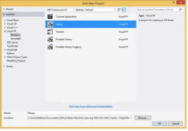
So, instead of a console application, we’ll work in a script. Let’s go into Visual Studio and add a new library project to our solution (see Figure 1-7), which we will name FSharp.
Figure 1-7. Adding an F# library project
It’s worth pointing that you have just added an F# project to a .NET solution with an existing C# project. F# and C# are completely interoperable and can talk to each other without problems—you don’t have to restrict yourself to using one language for everything. Unfortunately, oftentimes people think of C# and F# as competing languages, which they aren’t. They complement each other very nicely, so get the best of both worlds: Use C# for what C# is great at, and leverage the F# goodness for where F# shines!
In your new project, you should see now a file named Library1.fs; this is the F# equivalent of a .cs file. But did you also notice a file called script.fsx? .fsx files are script files; unlike .fs files, they are not part of the build. They can be used outside of Visual Studio as pure, free-standing scripts, which is very useful in its own right. In our current context, machine learning and data science, the usage I am particularly interested in is in Visual Studio: .fsx files constitute a wonderful “scratch pad” where you can experiment with code, with all the benefits of IntelliSense.
Let’s go to Script.fsx, delete everything in there, and simply type the following anywhere:
let x = 42
Now select the line you just typed and right click. On your context menu, you will see an option for “Execute in Interactive,” shown in Figure 1-8.
■
Tip
You can also execute whatever code is selected in the script file by using the keyboard shortcut
Alt + Enter. This is much faster than using the mouse and the context menu. A small warning to ReSharper
users: Until recently, ReSharper had the nasty habit of resetting that shortcut, so if you are using a version older
than 8.1, you will probably have to recreate that shortcut.
The F# Interactive window (which we will refer to as FSI most of the time, for the sake of brevity) runs as a session. That is, whatever you execute in the interactive window will remain in memory, available to you until you reset your session by right-clicking on the contents of the F# Interactive window and selecting “Reset Interactive Session.”
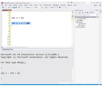
In this example, we simply create a variable x, with value 42. As a first approximation, this is largely similar to the C# statement var x = 42; There are some subtle differences, but we’ll discuss them later. Now that x “exists” in FSI, we can keep using it. For instance, you can type the following directly in FSI:
> x + 100;; val it : int = 142 >
Figure 1-9. Executing code live in F# Interactive
FSI “remembers” that x exists: you do not need to rerun the code you have in the .fsx file. Once it has been run once, it remains in memory. This is extremely convenient when you want to manipulate a somewhat large dataset. With FSI, you can load up your data once in the morning and keep coding, without having to reload every single time you have a change, as would be the case in C#.
You probably noted the mysterious ;; after x + 100. This indicates to FSI that whatever was typed until that point needs to be executed now. This is useful if the code you want to execute spans multiple lines, for instance.
■
Tip
If you tried to type F# code directly into FSI, you probably noticed that there was no IntelliSense. FSI
is a somewhat primitive development environment compared to the full Visual Studio experience. My advice in
terms of process is to type code in FSI only minimally. Instead, work primarily in an .fsx file. You will get all the
benefits of a modern IDE, with auto-completion and syntax validation, for instance. This will naturally lead you to
write complete scripts, which can then be replayed in the future. While scripts are not part of the solution build,
they are part of the solution itself, and can (should) be versioned as well, so that you are always in a position to
replicate whatever experiment you were conducting in a script.
Creating our First F# Script
Now that we have seen the basics of FSI, let’s get started. We will convert our C# example, starting with reading the data. First, we will execute a complete block of F# code to see what it does, and then we will examine it in detail to see how it all works. Let’s delete everything we currently have in Script.fsx, and write the F# code shown in Listing 1-10:
Listing 1-10. Reading data from file
open System.IO
type Observation = { Label:string; Pixels: int[] }
let toObservation (csvData:string) = let columns = csvData.Split(',') let label = columns.[0]
let pixels = columns.[1..] |> Array.map int { Label = label; Pixels = pixels }
let reader path =
let data = File.ReadAllLines path data.[1..]
|> Array.map toObservation
There is quite a bit of action going on in these few lines of F#. Before discussing how this all works, let’s run it to see the result of our handiwork. Select the code, right click, and pick “Run in Interactive.” After a couple of seconds, you should see something along these lines appear in the F# Interactive window:
>
type Observation = {Label: string; Pixels: int [];}
val observationFactory : csvData:string -> Observation val reader : path:string -> Observation []
val trainingPath : string = "-"+[58 chars]
val trainingData : Observation [] = [|{Label = "1";
Pixels =
[|0; 0; 0; 0; 0; 0; 0; 0; 0; 0; 0; 0; 0; 0; 0; 0; 0; 0; 0; 0; 0; 0; 0; 0; 0; 0; 0; 0; 0; 0; 0; 0; 0; 0; 0; 0; 0; 0; 0; 0; 0; 0; 0; 0; 0; 0; 0; 0; 0; 0; 0; 0; 0; 0; 0; 0; 0; 0; 0; 0; 0; 0; 0; 0; 0; 0; 0; 0; 0; 0; 0; 0; 0; 0; 0; 0; 0; 0; 0; 0; 0; 0; 0; 0; 0; 0; 0; 0; 0; 0; 0; 0; 0; 0; 0; 0; 0; 0; 0; 0; ...|];};
/// Output has been cut out for brevity here /// {Label = "3";
Pixels =
[|0; 0; 0; 0; 0; 0; 0; 0; 0; 0; 0; 0; 0; 0; 0; 0; 0; 0; 0; 0; 0; 0; 0; 0; 0; 0; 0; 0; 0; 0; 0; 0; 0; 0; 0; 0; 0; 0; 0; 0; 0; 0; 0; 0; 0; 0; 0; 0; 0; 0; 0; 0; 0; 0; 0; 0; 0; 0; 0; 0; 0; 0; 0; 0; 0; 0; 0; 0; 0; 0; ...|];}; ...|]
>
Basically, in a dozen lines of F#, we got all the functionality of the DataReader and Observation classes. By running it in F# Interactive, we could immediately load the data and see how it looked. At that point, we loaded an array of Observations (the data) in the F# Interactive session, which will stay there for as long as you want. For instance, suppose that you wanted to know the label of Observation 100 in the training set. No need to reload or recompile anything: just type the following in the F# Interactive window, and execute:
let test = trainingData.[100].Label;;
And that’s it. Because the data is already there in memory, it will just work.
Dissecting Our First F# Script
Now that we saw what these ten lines of code do, let’s dive into how they work:
open System.IO
This line is straightforward—it is equivalent to the C# statement using System.IO. Every .NET library is accessible to F#, so all the knowledge you accumulated over the years learning the .NET namespaces jungle is not lost—you will be able to reuse all that and augment it with some of the F#-specific goodies made available to you!
In C#, we created an Observation class to hold the data. Let’s do the same in F#, using a slightly different type:
type Observation = { Label:string; Pixels: int[] }
Boom—done. In one line, we created a record (a type specific to F#), something that is essentially an immutable class (and will appear as such if you call your F# code from C#), with two properties: Label and
Pixels. To use a record is then as simple as this:
let myObs = { Label = "3"; Pixels = [| 1; 2; 3; 4; 5 |] }
We instantiate an Observation by simply opening curly braces and filling in all its properties. F# automatically infers that what we want is an Observation, because it is the only record type that has the correct properties. We create an array of integers for Pixels by simply opening and closing an array with the symbols [| |] and filling in the contents.
Now that we have a container for the data, let’s read from the CSV file. In the C# example, we created a method, ReadObservations, and a DataReader class to hold it, but that class is honestly not doing much for us. So rather than creating a class, we’ll simply write a function reader, which takes one argument, path, and uses an auxiliary function to extract an Observation from a csv line:
let toObservation (csvData:string) = let columns = csvData.Split(',') let label = columns.[0]
let pixels = columns.[1..] |> Array.map int { Label = label; Pixels = pixels }
let reader path =
let data = File.ReadAllLines path data.[1..]
|> Array.map toFactory
Let’s begin with a high-level overview. Here is how our equivalent C# code looked (Listing 1-2):
private static Observation ObservationFactory(string data) {
var commaSeparated = data.Split(','); var label = commaSeparated[0];
return new Observation(label, pixels); }
There are a few obvious differences between C# and F#. First, F# doesn’t have any curly braces; F#, like other languages such as Python, uses whitespace to mark code blocks. In other words, white space is significant in F# code: when you see code indented by whitespace, with the same depth, then it belongs to the same block, as if invisible curly braces were around it. In the case of the reader function in Listing 1-10, we can see that the body of the function starts at let data ... and ends with |> Array.map observationFactory.
Another obvious high-level difference is the missing return type, or type declaration, on the function argument. Does this mean that F# is a dynamic language? If you hover over reader in the .fsx file, you’ll see the following hint show up: val reader : path:string -> Observation [], which denotes a function that takes a path, expected to be of type string, and returns an array of observations. F# is every bit as statically typed as C#, but uses a powerful type-inference engine, which will use every hint available to figure out all by itself what the correct types have to be. In this case, File.ReadAllLines has only two overloads, and the only possible match implies that path has to be a string.
In a way, this gives you the best of both worlds—you get all the benefits of having less code, just as you would with a dynamic language, but you also have a solid type system, with the compiler helping you avoid silly mistakes.
The other interesting difference between C# and F# is the missing return statement. Unlike C#, which is largely procedural, F# is expression oriented. An expression like let x = 2 + 3 * 5 binds the name x to an expression; when that expression is evaluated as (2 + 3 * 5 is 17), the value is bound to x. The same goes for a function: The function will evaluate to the value of the last expression. Here is a contrived example to illustrate what is happening:
let demo x y = let a = 2 * x let b = 3 * y let z = a + b
z // this is the last expression:
// therefore demo will evaluate to whatever z evaluates to.
Another difference you might have picked up on, too, is the lack of parentheses around the arguments. Let’s ignore that point for a minute, but we’ll come back to it a bit later in this chapter.
Creating Pipelines of Functions
Let’s dive in to the body of the read function. let data = File.ReadAllLines path simply reads all the contents of the file located at path into an array of strings, one per line, all at once. There’s no magic here, but it proves the point that we can indeed use anything made available in the .NET framework from F#, regardless of what language was used to write it.
data.[1..] illustrates the syntax for indexers in F#; myArray.[0] will return the first element of your array. Note the presence of a dot between myArray and the bracketed index! The other interesting bit of syntax here demonstrates array slicing; data.[1..] signifies “give me a new array, pulling elements from data starting at index 1 until the last one.” Similarly, you could do things like data.[5..10] (give me all elements from indexes 5 to 10), or data.[..3] (give me all elements until index 3). This is incredibly convenient for data manipulation, and is one of the many reasons why F# is such a nice language for data science.
In our example, we kept every element starting at index 1, or in other words, we dropped the first element of the array—that is, the headers.
The next step in our C# code involved extracting an Observation from each line using the
ObservationFactory method, which we did by using the following:
myData.Select(line => ObservationFactory(line));
The equivalent line in F# is as follows:
myData |> Array.map (fun line -> toObservation line)
■
Note
If you enjoy using LINQ in C#, I suspect you will really like F#. In many respects, LINQ is about
importing concepts from functional programming into an object-oriented language, C#. F# offers a much deeper
set of LINQ-like functions for you to play with. To get a sense for that, simply type “Array.” in .fsx, and see how
many functions you have at your disposal!
The second major difference is the mysterious symbol “|>”. This is known as the pipe-forward operator. In a nutshell, it takes whatever the result of the previous expression was and passes it forward to the next function in the pipeline, which will use it as the last argument. For instance, consider the following code:
let double x = 2 * x let a = 5
let b = double a let c = double b
This could be rewritten as follows:
let double x = 2 * x
let c = 5 |> double |> double
double is a function expecting a single argument that is an integer, so we can “feed” a 5 directly into it through the pipe-forward operator. Because double also produces an integer, we can keep forwarding the result of the operation ahead. We can slightly rewrite this code to look this way:
let double x = 2 * x let c =
5
|> double |> double
Our example with Array.map follows the same pattern. If we used the raw Array.map version, the code would look like this:
let transformed = Array.map (fun line -> toObservation line) data
Array.map expects two arguments: what transformation to apply to each array element, and what array to apply it to. Because the target array is the last argument of the function, we can use pipe-forward to “feed” an array to a map, like this:
data |> Array.map (fun line -> toObservation line)
Manipulating Data with Tuples and Pattern Matching
Now that we have data, we need to find the closest image from the training set. Just like in the C# example, we need a distance for that. Unlike C#, again, we won’t create a class or interface, and will just use a function:
let manhattanDistance (pixels1,pixels2) = Array.zip pixels1 pixels2
|> Array.map (fun (x,y) -> abs (x-y)) |> Array.sum
Here we are using another central feature of F#: the combination of tuples and pattern matching. A tuple is a grouping of unnamed but ordered values, possibly of different types. Tuples exist in C# as well, but the lack of pattern matching in the language really cripples their usefulness, which is quite unfortunate, because it’s a deadly combination for data manipulation.
There is much more to pattern matching than just tuples. In general, pattern matching is a mechanism with allows your code to simply recognize various shapes in the data, and to take action based on that. Here is a small example illustrating how pattern matching works on tuples:
let x = "Hello", 42 // create a tuple with 2 elements
let (a, b) = x // unpack the two elements of x by pattern matching printfn "%s, %i" a b
printfn "%s, %i" (fst x) (snd x)
Here we “pack” within x two elements: a string “Hello” and an integer 42, separated by a comma. The comma typically indicates a tuple, so watch out for this in F# code, as this can be slightly confusing at first. The second line “unpacks” the tuple, retrieving its two elements into a and b. For tuples of two elements, a special syntax exists to access its first and second elements, using the fst and snd functions.
■
Tip
You may have noticed that, unlike C#, F# does not use parentheses to define the list of arguments a
function expects. As an example,
add x y = x + yis how you would typically write an addition function. The
following function
tupleAdd (x, y) = x + yis perfectly valid F# code, but has a different meaning: It expects
a single argument, which is a fully-formed tuple. As a result, while
1 |> add 2is valid code,
1 |> tupleAdd 2will fail to compile—but
(1,2) |> tupleAddwill work.
This approach extends to tuples beyond two elements; the main difference is that they do not support
fst and snd. Note the use of the wildcard _ below, which means “ignore the element in 2nd position”:
let y = 1,2,3,4 let (c,_,d,e) = y
printfn "%i, %i, %i" c d e
Let’s see how this works in the manhattanDistance function. We take the two arrays of pixels (the images) and apply Array.zip, creating a single array of tuples, where elements of the same index are paired up together. A quick example might help clarify:
let array1 = [| "A";"B";"C" |] let array2 = [| 1 .. 3 |]
Running this in FSI should produce the following output, which is self-explanatory:
val zipped : (string * int) [] = [|("A", 1); ("B", 2); ("C", 3)|]
So what the Manhattan distance function does is take two arrays, pair up corresponding pixels, and for each pair it computes the absolute value of their difference and then sums them all up.
Training and Evaluating a Classifier Function
Now that we have a Manhattan distance function, let’s search for the element in the training set that is closest to the image we want to classify:
let train (trainingset:Observation[]) = let classify (pixels:int[]) = trainingset
|> Array.minBy (fun x -> manhattanDistance x.Pixels pixels) |> fun x -> x.Label
classify
let classifier = train training
train is a function that expects an array of Observation. Inside that function, we create another function, classify, which takes an image, finds the image that has the smallest distance from the target, and returns the label of that closest candidate; train returns that function. Note also how while
manhattanDistance is not part of the arguments list for the train function, we can still use it inside it; this is known as “capturing a variable into a closure,” using within a function a variable whose scope is not defined inside that function. Note also the usage of minBy (which doesn’t exist in C# or LINQ), which conveniently allows us to find the smallest element in an array, using any arbitrary function we want to compare items to each other.
Creating a model is now as simple as calling train training. If you hover over classifier, you will see it has the following type:
val classifier : (int [] -> string)
What this tells you is that classifier is a function, which takes in an array of integers (the pixels of the image you are trying to classify), and returns a string (the predicted label). In general, I highly recommend taking some time hovering over your code and making sure the types are what you think they are. The F# type inference system is fantastic, but at times it is almost too smart, and it will manage to figure out a way to make your code work, just not always in the way you anticipated.
And we are pretty much done. Let’s now validate our classifier:
let validationPath = @" PATH-ON-YOUR-MACHINE\validationsample.csv" let validationData = reader validationPath
validationData
|> Array.averageBy (fun x -> if model x.Pixels = x.Label then 1. else 0.) |> printfn "Correct: %.3f"
And that’s it. In thirty-ish lines of code, in a single file, we have all of the required code in its full glory. There is obviously much more to F# than what we just saw in this short crash course. However, at this point, you should have a better sense of what F# is about and why it is such a great fit for machine learning and data science. The code is short but readable, and works great for composing data-transformation pipelines, which are an essential activity in machine learning. The F# Interactive window allows you to load your data in memory, once, and then explore the data and modeling ideas, without wasting time reloading and recompiling. That alone is a huge benefit—but we’ll see much more about F#, and how to combine its power with C#, as we go further along in the book!
Improving Our Model
We implemented the Dumbest Model That Could Possibly Work, and it is actually performing pretty well—93.4% correct. Can we make this better?
Unfortunately, there is no general answer to that. Unless your model is already 100% correct in its predictions, there is always the possibility of making improvements, and there is only one way to know: try things out and see if it works. Building a good predictive model involves a lot of trial and error, and being properly set up to iterate rapidly, experiment, and validate ideas is crucial.
What directions could we explore? Off the top of my head, I can think of a few. We could
• tweak the distance function. The Manhattan distance we are using here is just one of
many possibilities, and picking the “right” distance function is usually a key element in having a good model. The distance function (or cost function) is essentially how you convey to the machine what it should consider to be similar or different items in its world, so thinking this through carefully is very important.
• search for a number of closest points instead of considering just the one closest
point, and take a “majority vote.” This could make the model more robust; looking at more candidates could reduce the chance that we accidentally picked a bad one. This approach has a name—the algorithm is called “K Nearest Neighbors,” and is a classic of machine learning.
• do some clever trickery on the images; for instance, imagine taking a picture,
but shifting it by one pixel to the right. If you compared that image to the original version, the distance could be huge, even though they ARE the same image. One way we could compensate for that problem is, for instance, by using some blurring. Replacing each pixel with the average color of its neighbors could mitigate “image misalignment” problems.
I am sure you could think of other ideas, too. Let’s explore the first one together.
Experimenting with Another Definition of Distance
Let’s begin with the distance. How about trying out the distance you probably have seen in high school, pedantically known as the Euclidean distance? Here is the math for that distance:
Dist X Y
(
,)
=(
x1-y1)
+(
x -y)
+ +(
xn-yn)
2
2 2
2 2
This simply states that the distance between two points X and Y is the square root of the sum of the difference between each of their coordinates, squared up. You have probably seen a simplified version of this formula, stating that if you take two points on a plane, X = (x1, x2) and Y = (y1, y2), their Euclidean distance is:
Dist X Y
(
,)
=(
x1-y1)
+(
x -y)
2
2 2 2
In case you are more comfortable with code than with math, here is how it would look in F#:
let euclideanDistance (X,Y) = Array.zip X Y
|> Array.map (fun (x,y) -> pown (x-y) 2) |> Array.sum
|> sqrt
We take two arrays of floats as input (each representing the coordinates of a point), compute the difference for each of their elements and square that, sum, and take the square root. Not very hard, and pretty clear!
A few technical details should be mentioned here. First, F# has a lot of nice mathematical functions built in, which you would typically look for in the System.Math class. sqrt is such a function—isn’t it nice to be able to write let x = sqrt 16.0 instead of var x = Math.Sqrt(16)? pown is another such function; it is a specialized version of “raise to the nth power” for cases when the exponent is an integer. The general version is the ** operator, as in let x = 2.0 ** 4.0; pown will give you significant performance boosts when you know the exponent is an integer.
Another detail: The distance function we have here is correct, but technically, for our purposes, we can actually drop the sqrt from there. What we need is the closest point, and if 0 <= A < B, then sqrt A < sqrt B. So rather than incur the cost of that operation, let’s drop it. This also allows us to operate on integers, which is much faster than doubles or floats.
Factoring Out the Distance Function
If our goal is to experiment with different models, it’s probably a good time to do some refactoring. We want to swap out different pieces in our code and see what the impact is on the prediction quality. Specifically, we want to switch distances. The typical object-oriented way to do that would be to extract an interface, say
IDistance, and inject that into the training (which is exactly what we did in the C# sample). However, if you really think about it, the interface is total overkill—the only thing we need is a function, which takes two points as an input and returns an integer, their distance from each other. Here is how we could do it:
Listing 1-11. Refactoring the distance
type Distance = int[] * int[] -> int
let manhattanDistance (pixels1,pixels2) = Array.zip pixels1 pixels2
|> Array.map (fun (x,y) -> abs (x-y)) |> Array.sum
let euclideanDistance (pixels1,pixels2) = Array.zip pixels1 pixels2
let train (trainingset:Observation[]) (dist:Distance) = let classify (pixels:int[]) =
trainingset
|> Array.minBy (fun x -> dist (x.Pixels, pixels)) |> fun x -> x.Label
classify
Instead of an interface, we create a type Distance, which is a function signature that expects a pair of pixels and returns an integer. We can now pass any Distance we want as an argument to the train function, which will return a classifier using that particular distance. For instance, we can train a classifier with the manhattanDistance function, or the euclideanDistance function (or any other arbitrary distance function, in case we want to experiment further), and compare how well they perform. Note that this would all be perfectly possible in C# too: Instead of creating an interface IDistance, we could simply use
Func<int[],int[],int>. This is how our code would look:
Listing 1-12. Functional C# example
public class FunctionalExample {
private IEnumerable<Observation> data;
private readonly Func<int[], int[], int> distance;
public FunctionalExample(Func<int[], int[], int> distance) {
this.distance = distance; }
public Func<int[], int[], int> Distance {
get { return this.distance; } }
public void Train(IEnumerable<Observation> trainingSet) {
this.data = trainingSet; }
public string Predict(int[] pixels) {
Observation currentBest = null; var shortest = Double.MaxValue;
foreach (Observation obs in this.data) {
{
This approach, which focuses on composing functions instead of objects, is typical of what’s called a functional style of programming. C#, while coming from object-oriented roots, supports a lot of functional idioms. Arguably, pretty much every feature and innovation that has made its way into C# since version 3.5 (LINQ, Async, ...) has been borrowed from functional programming. At this point, one could describe C# as a language that is object oriented first, but supports functional idioms, whereas F# is a functional programming language first, but can accommodate an object-oriented style as well. Throughout this book, we will in general emphasize a functional style over an object-oriented one, because in our opinion it fits much better with machine learning algorithms than an object-oriented style does, and also because, more generally, code written in a functional style offers serious benefits.
In any case, we are set up to see whether our idea is a good one. We can now create two models and compare their performance:
The nice thing here is that we don’t have to reload the dataset in memory; we simply modify the script file, select the section that contains new code we want to run, and run it. If we do that, we should see that the new model, euclideanModel, correctly classifies 94.4% of the images, instead of 93.4% for the
manhattanModel. Nice! We just squeezed in a 1% improvement. 1% might not sound like much, but if you are already at 93.4%, you just reduced your error from 6.6% to 5.6%, a gain of around 15%.
So, What Have We Learned?
We covered quite a bit of ground in this chapter! On the machine learning front, you are now familiar with a few key concepts, as well as with the methodology. And if you are new to F#, you have now written your first piece of F# code!
Let’s review some of the main points, starting with the machine learning side.
First, we discussed cross-validation, the process of using separate datasets for training and validation, setting apart some of the data to evaluate the quality of your prediction model. This is a crucial process on many levels. First, it provides you with a baseline, a “ground truth” that guides your experimentation. Without a validation set, you cannot make judgments on whether a particular model is better than another. Cross-validation allows you to measure quality scientifically. It plays a role somewhat analogous to an automated test suite, warning you when your development efforts are going off the rails.
Once your cross-validation setup is in place, you can try to experiment, selecting models or directions to investigate on quantifiable grounds. The trial-and-error approach is an essential part of “doing machine learning.” There is no way to know beforehand if a particular approach will work well, so you will have to try it out on the data to see by yourself, which makes it very important to set yourself up for success and embrace “reproducible research” ideas. Automate your process as much as possible with scripts, and use source control liberally so that at any given point you can replicate every step of your model without human intervention. In general, set yourself up so that you can easily change and run code.
What to Look for in a Good Distance Function
In our digit-recognizer exploration, we saw that a small change in what distance we used significantly improved our model. At the heart of most (every?) machine learning models, there is a distance function. All the learning process boils down to is the computer attempting to find the best way possible to fit known data to a particular problem – and the definition of “best fit” is entirely encapsulated in the distance function. In a way, it is the translation of your goals from a human form into a statement that is understandable by a machine, stated using mathematics. The distance function is also frequently called the cost function; thinking in cost emphasizes more what makes a bad solution bad, and what penalty to use so as to avoid selecting bad solutions.
In my experience, it is always worthwhile to take the time to think through your cost function. No matter how clever an algorithm you use, if the cost function is flawed, the results will be terrible. Imagine a dataset of individuals that includes two measurements: height in feet and weight in pounds. If we were to search for the “most similar” individuals in our dataset, along the lines of what we did for images, here is what will happen: While heights are typically in the 5 to 6 feet range, weights are on a wider and higher scale, say, 100 to 200 pounds. As a result, directly computing a distance based on these two measurements will essentially ignore differences in height, because a 1 foot difference will be equivalent to a 1 pound difference. One way to address this is to transform all features to make sure they are on consistent scales, a process known as “normalization,” a topic we’ll discuss in more detail later. Fortunately, all pixels are encoded on an identical scale, and we could ignore that problem here, but I hope this example of “Distance Gone Wrong” gives you a sense of why it is worth giving your distance function some thought!
This is also one of those cases where the proper mathematical definitions are actually useful. If you dig back your math notes from way back in school, you’ll see that a distance function (sometimes also called a metric by mathematicians) is defined by a few properties:
• Distance(A,B) > 0 (there is no negative distance)
• Distance(A,B) = Distance(B,A) (symmetry: going from A to B should be the same
length as going from B to A)
• Distance(A,B) <= Distance(A,C) + Distance(C,B) (“Triangle inequality”: there is no
shorter distance between two points than direct travel)
We just looked at two distances in this chapter, but there is a wide variety of functions that satisfy these properties, each of which defines similarity in a different manner. For that matter, the cost function in a model doesn’t need to satisfy all these properties, but in general, if it doesn’t, you might want to ask yourself what unintended side effects could arise because of it. For instance, in the initial example with the Manhattan distance, if we had omitted the absolute value, we would be blatantly violating both rule 1 (non-negative distance) and rule 3 (symmetry). In some case, there are good reasons to take liberties and use a function that is not a metric, but when that happens, take an extra minute to think through what could possibly go wrong!
Models Don’t Have to Be Complicated
Finally, I hope what came through is that effective models don’t have to be complicated! Whether in C# or F#, both classifiers were small and used fairly simple math. Of course, some complex models may give you amazing results, too, but if you can get the same result with a simple model that you can understand and modify easily, then why not go for easy?
This is known as Occam’s Razor, named after William of Ockham, a medieval philosopher. Occam’s Razor follows a principle of economy. When trying to explain something, when choosing between multiple models that could fit, pick the simplest one. Only when no simple explanation works should you go for complicated models.
In the same vein, we implemented first “the simplest thing that could possibly work” here, and I strongly encourage you to follow that approach. If you don’t, here is what will probably happen: You will start implementing a few ideas that could work; they will spark new ideas, so you will soon have a bunch of half-baked prototypes, and will go deeper and deeper in the jungle, without a clear process or method. Suddenly, you will realize you have spent a couple of weeks coding away, and you are not quite sure whether anything works or where to go from there. This is not a good feeling. Time box yourself and spend one day (or one week, or one hour, whatever is realistic given your problem) and build an end-to-end model with the dumbest, simplest possible prediction model you can think of. It might actually turn out to be good enough, in which case you won’t have wasted any time. And if it isn’t good enough, by that point you will have a proper harness, with data integration and cross-validation in place, and you will also likely have uncovered whatever unexpected nastiness might exist in your dataset. You will be in a great place to enter the jungle.
Why F#?
If this was your first exposure to F#, you might have wondered initially why I would introduce that language, and not stick with C#. I hope that the example made clear why I did! In my opinion, while C# is a great language, F# is a fantastic fit for machine learning and data exploration. We will see more of F# in further chapters, but I hope some of these reasons became clear in this chapter.