Full Terms & Conditions of access and use can be found at
http://www.tandfonline.com/action/journalInformation?journalCode=ubes20
Download by: [Universitas Maritim Raja Ali Haji], [UNIVERSITAS MARITIM RAJA ALI HAJI
TANJUNGPINANG, KEPULAUAN RIAU] Date: 11 January 2016, At: 20:35
Journal of Business & Economic Statistics
ISSN: 0735-0015 (Print) 1537-2707 (Online) Journal homepage: http://www.tandfonline.com/loi/ubes20
Do Central Bank Liquidity Facilities Affect
Interbank Lending Rates?
Jens H. E. Christensen, Jose A. Lopez & Glenn D. Rudebusch
To cite this article: Jens H. E. Christensen, Jose A. Lopez & Glenn D. Rudebusch (2014) Do Central Bank Liquidity Facilities Affect Interbank Lending Rates?, Journal of Business & Economic Statistics, 32:1, 136-151, DOI: 10.1080/07350015.2013.858631
To link to this article: http://dx.doi.org/10.1080/07350015.2013.858631
Accepted author version posted online: 13 Nov 2013.
Submit your article to this journal
Article views: 345
View related articles
Do Central Bank Liquidity Facilities Affect
Interbank Lending Rates?
Jens H. E. C
HRISTENSEN, Jose A. L
OPEZ, and Glenn D. R
UDEBUSCHFederal Reserve Bank of San Francisco, San Francisco, CA 94105 ([email protected]; [email protected]; [email protected])
In response to the global financial crisis that started in August 2007, central banks provided extraordinary amounts of liquidity to the financial system. To investigate the effect of central bank liquidity facilities on term interbank lending rates near the start of the crisis, we estimate a six-factor arbitrage-free model of U.S. Treasury yields, financial corporate bond yields, and term interbank rates. This model can account for fluctuations in the term structure of credit and liquidity spreads observed in the data. A significant shift in model estimates after the announcement of the liquidity facilities suggests that these central bank actions did help lower the liquidity premium in term interbank rates.
KEY WORDS: Arbitrage-free yield curve modeling; Financial crisis; Kalman filter; LIBOR.
1. INTRODUCTION
In early August 2007, amid declining prices and credit ratings for U.S. mortgage-backed securities and other forms of struc-tured credit, international money markets came under severe stress. Short-term funding rates in the interbank market rose sharply relative to yields on comparable-maturity government securities. For example, the 3-month U.S. dollar London inter-bank offered rate (LIBOR) jumped from an average of only 20 basis points higher than the 3-month U.S. Treasury yield dur-ing the first 7 months of 2007 to an average of over 110 basis points higher during the final 5 months of the year. This enlarged spread was also remarkable for persisting into 2008.
LIBOR rates are widely used as reference rates in financial instruments, including derivatives contracts, variable-rate home mortgages, and corporate notes, so their unusually high levels in 2007 and 2008 appeared likely to have widespread adverse financial and macroeconomic repercussions. (As a convenient redundancy, we follow the literature in referring to “LIBOR rates.”) To limit these adverse effects, central banks around the world established an extraordinary set of lending facilities that were intended to increase financial market liquidity and ease strains in term interbank funding markets, especially at maturi-ties of a few months or more. Monetary policy operations typi-cally focus on an overnight or very short term interbank lending rate. However, on December 12, 2007, the Bank of Canada, the Bank of England, the European Central Bank (ECB), the Fed-eral Reserve, and the Swiss National Bank jointly announced a set of measures designed to address elevated pressures in term funding markets. These measures included foreign exchange swap lines established by the Federal Reserve with the ECB and the Swiss National Bank to provide U.S. dollar funding in Europe. The Federal Reserve also announced a new Term Auc-tion Facility, or TAF, to provide depository instituAuc-tions with a source of term funding. The TAF term loans were secured with various forms of collateral and distributed through an auction. (For further details on this facility, see Armantier, Krieger, and McAndrews2008.)
The TAF and similar term lending facilities by other central banks were not monetary policy actions as traditionally defined.
(The Federal Reserve, in its normal operations, tries to hit a daily target for the federal funds rate, which is the overnight interest rate for interbank lending of bank reserves. The central bank liquidity facilities were not intended to alter the current level or the expected future path for the funds rate or the overall level of bank reserves, i.e., the term lending was sterilized by sales of Treasury securities.) Instead, these central bank actions were meant to improve the distribution of reserves and liquidity by targeting a narrow market-specific funding problem. The press release introducing the TAF described its purpose in this way: “By allowing the Federal Reserve to inject term funds through a broader range of counterparties and against a broader range of collateral than open market operations, this facility could help promote the efficient dissemination of liquidity when the unsecured interbank markets are under stress” (Federal Reserve Board December 12,2007).
This article assesses the effect of the establishment of these extraordinary central bank liquidity facilities on the interbank lending market and, in particular, on term LIBOR spreads over Treasury yields. In theory, the provision of central bank liquidity could lower the liquidity premium on interbank debt through a variety of channels. On the supply side, banks that have a greater assurance of meeting their own unforeseen liquidity needs over time should be more willing to extend term loans to other banks. In addition, creditors should also be more willing to provide funding to banks that have easy and dependable access to funds, since there is a greater reassurance of timely repayment. On the demand side, with a central bank liquidity backstop, banks should be less inclined to borrow from other banks to satisfy any precautionary demand for liquid funds because their future idiosyncratic demands for liquidity over time can be met via the backstop. However, assessing the relative importance of these channels is difficult. Furthermore, judging the efficacy of central bank liquidity
© 2014American Statistical Association Journal of Business & Economic Statistics January 2014, Vol. 32, No. 1 DOI:10.1080/07350015.2013.858631 Color versions of one or more of the figures in the article can be found online atwww.tandfonline.com/r/jbes.
136
facilities in lowering the liquidity premium is complicated because LIBOR rates, which are for unsecured bank deposits, also include a credit risk premium for the possibility that the borrowing bank may default; see He and Xiong(2012) for a model of these interrelated premia. The elevated LIBOR rates during the financial crisis likely reflected both higher credit risk and liquidity premiums, so any assessment of the effect of the recent extraordinary central bank liquidity provision must attempt to capture fluctuations in both credit and liquidity risk.
To analyze the effectiveness of the central bank liquidity fa-cilities in reducing interbank lending pressures, we use a multi-factor arbitrage-free (AF) representation of the term structure of interest rates and bank credit risk. Specifically, we estimate an affine AF term structure representation of U.S. Treasury yields, the yields on bonds issued by financial institutions, and term LIBOR rates using weekly data from 1995 to midyear 2008. For tractability, the model uses the AF Nelson–Siegel (AFNS) structure. Christensen, Diebold, and Rudebusch(2011)showed that a three-factor AFNS model fits and forecasts the Treasury yield curve very well. In this article, we incorporate three addi-tional factors: two factors that capture bank debt risk dynamics, as in Christensen and Lopez(2012), and a third factor specific to LIBOR rates. The resulting six-factor representation provides AF joint pricing of treasury yields, financial corporate bond yields, and LIBOR rates. This structure allows us to decompose movements in LIBOR rates into changes in bank debt spreads and changes in a factor specific to the interbank market (i.e., a model-implied LIBOR factor) that should capture liquidity issues more closely. We can also conduct hypothesis testing and counterfactual analysis related to the introduction of the central bank liquidity facilities.
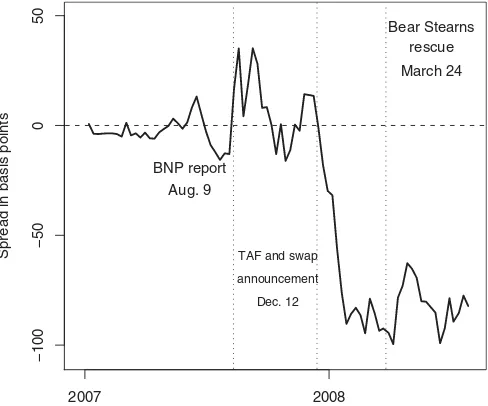
Our results support the view that the central bank liquidity facilities established in December 2007 helped lower LIBOR rates. Specifically, the parameters governing the term LIBOR factor within the model are shown to change after the introduc-tion of the liquidity facilities, suggesting that the behavior of this factor and thus of the interbank market was directly affected by these facilities. To quantify this effect, we use the model to construct a counterfactual path for the 3-month LIBOR rate by assuming that the LIBOR factor remained constant at its histor-ical average after the introduction of the liquidity facilities. Our analysis suggests that the counterfactual 3-month LIBOR rate averaged significantly higher—on the order of 70 basis points higher—than the observed rate from December 2007 through the middle of 2008. Correspondingly, as shown inFigure 1, the difference between the observed and our model-implied coun-terfactual 3-month LIBOR rates quickly turned negative and reached approximately −75 basis points after the announce-ment, where it stayed for the remainder of our sample through July 2008. This result suggests that if the central bank liquidity facilities had not been created, the 3-month LIBOR rate would have been substantially higher. Further analysis of the model-implied LIBOR factor suggests that liquidity dynamics in the interbank market were even more dramatically affected by the various financial firm defaults in September 2008 and did not return to precrisis levels until the fall of 2009 with the assistance of many central bank and government support programs.
There are two recent research literatures particularly relevant to our analysis. First, in terms of methodology, our empirical
8 0 0 2 7
0 0 2
−100
−50
0
50
Spread in
b
asis points BNP report Aug. 9
TAF and swap
announcement Dec. 12
Bear Stearns rescue March 24
Figure 1. Difference between the 3-month LIBOR rate and coun-terfactual. This figure shows the observed 3-month LIBOR rate minus the model-implied counterfactual path generated by fixing the LIBOR-specific factor at its historical average prior to December 14, 2007, in effect neutralizing the idiosyncratic effects in the LIBOR market. The illustrated period starts at the beginning of 2007, while the model estimation sample covers the period from January 6, 1995 to July 25, 2008.
model is similar to earlier factor models of LIBOR rates, notably Collin-Dufresne and Solnik (2001)and Feldh¨utter and Lando
(2008). The latter, for example, incorporated a LIBOR rate in
a six-factor AF model of Treasury, swap, and corporate yields. They used two factors to describe Treasury yields, two factors for the credit spreads of financial corporate bonds, one factor for LIBOR rates, and one factor for swap rates—with all factors as-sumed to be independent. Although similar, our six-factor model allows for complete dynamic interactions among the various fac-tors and includes a broader range of maturities in the estimation. A second relevant literature, of course, is the ongoing anal-ysis of the recent financial crisis. Notably, with respect to the interbank market, McAndrews, Sarkar, and Wang(2008), Taylor and Williams(2009), Thornton(2011), and Wu(2011) exam-ined the effect of central bank liquidity facilities on the liquidity premium in LIBOR by controlling for movements in credit risk as measured by credit default swap (CDS) prices for the bor-rowing banks and other related credit instruments in standard event-study regressions. (There are also recent related theoreti-cal analysis of liquidity in the interbank lending market, as de-scribed in Allen, Carletti, and Gale2009.) Unfortunately, based on only differences in the specifications of their regressions, these studies disagree about the effectiveness of the central bank actions. Studies using firm-specific data on the interbank mar-ket, such as Angelini, Nobili, and Picillo(2011)and Gefang, Koop, and Potter(2011), also reach different empirical conclu-sions. Therefore, we employ a very different methodology that provides a more complete accounting of the dynamics of credit and liquidity risk premia.
The remainder of the article is structured as follows. The next section presents our data and details the structure of our empir-ical six-factor AF term structure model. Section 3 presents our
estimation method and model estimates, and Section 4 focuses on the financial crisis that started in August 2007. It describes the central bank liquidity facilities established and the subse-quent interest rate movements through the lens of our estimated model; in particular, testing for a structural break in the data and conducting a counterfactual exercise. Section 5 concludes.
2. AN EMPIRICAL MODEL OF TREASURY, BANK, AND LIBOR YIELDS
In this section, we describe the data from the three finan-cial markets of interest to our analysis and introduce an affine AF joint model of Treasury yields, financial bond yields, and LIBOR rates. It should be noted that this model is of reduced form, such that the spreads between the Treasury and financial yields are not modeled explicitly as credit and liquidity premia. Instead, we assume that these spreads are representations of the underlying credit and liquidity risk factors in these markets.
2.1 Three Financial Markets
Treasury securities, financial corporate bonds, and interbank term lending contracts are closely related debt instruments but differ in their relative amounts of credit and liquidity risk. Trea-sury securities are generally considered to be free from credit risk and are the most liquid debt instruments available. In our empirical work, we use 708 weekly observations (Fridays) from January 6, 1995 to July 25, 2008, on zero-coupon Treasury yields with maturities of 3, 6, 12, 24, 36, 60, 84, and 120 months, as described by G¨urkaynak, Sack, and Wright(2007). (We here limit our sample to July 2008 and encompass only the first year of the financial crisis for two reasons. During this period, the Federal Reserve’s liquidity operations were being sterilized, so they altered the composition and not the size of the Federal Reserve’s balance sheet. Also, after the end of our sample, there were additional policy actions, such as the Tem-porary Liquidity Guarantee Program administered by the FDIC that provided government insurance for bank debt, that have important implications for bank credit and liquidity risk, but do not involve direct injections of liquidity. This limited sample allows us to get a cleaner reading on just the effect of the Fed-eral Reserve’s liquidity facilities. See Section 4.2 for estimation results over a longer time period.) Prices for unsecured lending of U.S. dollars at various maturities between banks are given by LIBOR rates, which are determined each business morning by a British Bankers’ Association (BBA) survey of a panel of large London-based banks. (The BBA discards the four highest and four lowest quotes and takes the average of the remaining eight quotes, which becomes the LIBOR rate for that specific term deposit on that day. Further details are available on the BBA’s websitewww.bbalibor.com.) In the credit risk literature (e.g., Collin-Dufresne and Solnik2001), LIBOR rates are often considered on par with AA-rated corporate bond rates since the BBA survey panel of banks is reviewed and revised as necessary to maintain high credit quality. Our LIBOR data consist of the 3, 6, and 12 month maturities. (Appendix A describes the conver-sion of the quoted LIBOR rates into continuously compounded yields.) Please note that although concerns have been expressed about the integrity of LIBOR fixings during the crisis, we
as-1996 1998 2000 2002 2004 2006 2008
−50
0
5
0
100
150
Spread in
b
asis points
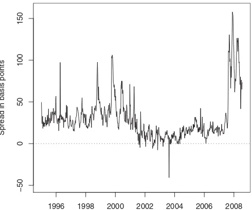
Figure 2. Spread of 3-month LIBOR rate over the Treasury yield. This figure shows the weekly spread of the 3-month LIBOR rate over the 3-month treasury bond yield from January 6, 1995 to July 25, 2008.
sume that such effects are part of the LIBOR market dynamics captured in the model.
Figure 2 illustrates the spread of the 3-month LIBOR rate
over the 3-month Treasury yield. Both the size and duration of this elevated spread in 2007 and 2008 clearly stand out as ex-ceptional. A key date is August 9, 2007, which marks the start of the turmoil in financial markets and the jump in LIBOR rates. An important trigger for the financial crisis and the tightening of the money markets was the announcement by the French bank BNP Paribas that it would suspend redemptions from three of its investment funds. (The BNP Paribas press release stated that “the complete evaporation of liquidity in certain market seg-ments of the U.S. securitization market has made it impossible to value certain assets fairly regardless of their quality or credit rating. . .during these exceptional times, BNP Paribas has de-cided to temporarily suspend the calculation of the net asset value as well as subscriptions/redemptions.” ) The mean spread in our sample prior to August 10, 2007 is about 25 basis points, while after that date, the mean spread is 98 basis points. (Data on the LIBOR-Treasury spread and the eurodollar-Treasury (or TED) yield spread can be obtained earlier than the 1995 start of our estimation sample, which is determined by the availability of bank debt rates. Even with respect to these earlier periods, the spreads observed during the recent episode stands out as atypically large.) Fluctuations in the LIBOR-Treasury spread are commonly attributed to movements in credit and liquidity risk premia. (The LIBOR-treasury spread is also affected by changes in the “convenience yield” for holding treasury secu-rities; therefore, Feldh¨utter and Lando(2008)and others used swap rates as an alternative riskless rate benchmark that is free from idiosyncratic treasury movements. However, because we focus on the dynamic interactions between bank bond yields and LIBOR rates, the choice of the risk-free rate is not an issue for our analysis. Also note that seasonality issues, as in Neely and Winters(2006), should not be an issue for our analysis since our LIBOR rates have maturities greater than 1 month.) The credit risk premium compensates for the possibility that the borrowing
bank will default, while the liquidity risk premium is compen-sation for tying up funds in loans that—unlike liquid Treasury securities—cannot easily be unwound before they mature.
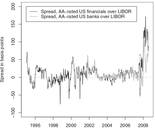
To examine the extent to which the observed jump in LIBOR rates was due to increased credit or liquidity risk, our empirical analysis compares these rates with yields on the unsecured bonds of U.S. financial institutions. We obtain zero-coupon yields on the bond debt of U.S. banks and financial corporations from Bloomberg at the eight Treasury maturities listed above. Our empirical model estimates the amount of risk associated with this financial debt by pooling across five different categories: A-rated and AA-rated financial corporate debt, and BBB-, A-, and AA-rated bank debt. (Appendix A describes the conversion of the reported interest rates into continuously compounded yields. These are the fair-value, zero-coupon curves provided by Bloomberg.) Yields for the first four types of debt are avail-able for our entire sample, while yields on AA-rated bank debt are only available after August 2001. At comparable maturities, LIBOR rates and yields on AA-rated bank debt should be very similar since they both represent the price of lending unsecured funds to such institutions. Indeed, for much of our sample, these rates are almost identical. As shown inFigure 3, at a 3-month maturity, the spread of the AA-rated bank debt yield over the LIBOR rate and the spread of the AA-rated financial corpo-rate debt yield over the LIBOR corpo-rate are typically very close to zero on average. Furthermore, most deviations—say, in 2001 and 2002—were short-lived. Therefore, financial bond debt and interbank loans appear to have had very similar credit and liquid-ity risk spreads, and we will use this relationship to control for broader credit risk dynamics within our modeling framework. Of course, there was a persistent and exceptional deviation that started at the end of 2007 during which the LIBOR rates fell below the yield on comparable financial corporate debt. We
pro-1996 1998 2000 2002 2004 2006 2008
−100
−50
0
50
100
150
200
Spread in
b
asis points
Spread, AA−rated US financials over LIBOR Spread, AA−rated US banks over LIBOR
Figure 3. Spreads of 3-month bank debt yields over LIBOR rates. This figure shows the yield spread on 3-month bonds issued by AA-rated U.S. banks over the 3 month LIBOR rate and the similar spread for AA-rated U.S. financial firms. The data for financial firms are from January 6, 1995 to July 25, 2008, while the data for banks start on September 21, 2001.
vide empirical evidence in Section 5 that therelativelylow rate on interbank borrowing after December 12, 2007 reflected the extraordinary commitment by central banks to provide liquidity to the interbank market.
2.2 Six-Factor AFNS Model
In this section, we introduce a joint affine, AF model of Treasury yields, financial bond yields, and LIBOR rates. To begin, letrT
t denote the risk-free short rate used for discounting
the cash flows from Treasury bonds. By implication, Treasury zero-coupon bond prices are given by
Pt(τ)=E Q t
e−
t+τ t rTsds,
where theQnotation refers to the risk-neutral probability mea-sure used for asset pricing. To price corporate bonds, we work within the reduced-form credit risk modeling framework un-der the assumption of “recovery of market value (RMV);” see Lando(1998)as well as Duffie and Singleton(1999)for details. Denote the default intensity by λQt and the recovery rate by
πtQ. Under the RMV assumption, the price of a representative
zero-coupon corporate bond is given by
Vt(τ)=EtQ
e−
t+τ t (rsT+(1−π
Q s )λQs)ds.
Since the loss rate (1−πtQ) and the default intensityλ Q t only
appear as a product under the RMV assumption, we replace the product (1−πQ
s )λ Q
s by the instantaneous credit spread, denoted
byst, without any loss of generality.
Following Duffie and Kan (1996), affine AF term structure models have been very popular, especially because yields on zero-coupon bonds like the two described above are conve-nient linear functions of underlying latent factors with factor loadings that can be calculated from a system of ordinary dif-ferential equations. To estimate such models, researchers have employed a variety of techniques; notably, Christensen, Diebold, and Rudebusch(2011)imposed general level, slope, and cur-vature factor loadings that are derived from the popular Nelson and Siegel(1987)yield curve to obtain an AFNS model. They showed that such a model fits and forecasts the term structure of Treasury yields quite well over time and can be estimated in a straightforward and robust fashion.
In this article, we show that an AFNS model can be read-ily estimated for a joint representation of treasury, bank bond, and LIBOR yields. Researchers have typically found that three factors—frequently referred to as level, slope, and curvature— are sufficient to model the time variation in the cross-section of nominal Treasury bond yields (e.g., Litterman and Scheinkman
1991). Similarly, we use a three-factor representation for trea-sury yields. The most general joint model of Treatrea-sury, bank bond, and LIBOR rates would add three more factors for the bank bond yield curve and another three for the LIBOR rates of various maturities. However, this nine-factor model is un-likely to be the most parsimonious empirical representation, for as noted in the previous section, movements in Treasury, bank bond, and LIBOR rates all share common elements.
Some evidence on the number of additional factors required to capture variation in financial bond yields can be obtained
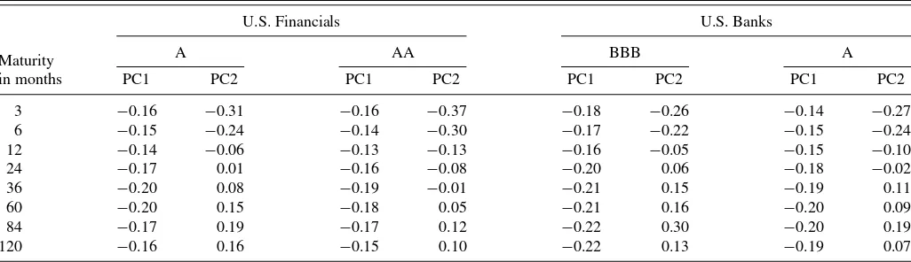
Table 1. Loadings on the first two principal components of credit spreads
U.S. Financials U.S. Banks
A AA BBB A
Maturity
in months PC1 PC2 PC1 PC2 PC1 PC2 PC1 PC2
3 −0.16 −0.31 −0.16 −0.37 −0.18 −0.26 −0.14 −0.27
NOTE: This table reports the loadings of each maturity on the first (PC1) and second (PC2) principal components for the zero-coupon credit spreads for A- and AA-rated U.S. financial firms and BBB- and A-rated U.S. banks covering the period from January 6, 1995 to July 25, 2008. The analysis is based on 32 time series, each with 708 weekly observations.
from their principal components. We subtract the bond yields for the four categories of debt that are available for our complete sample (i.e., A-rated and AA-rated financial corporate debt and BBB- and A-rated bank debt) from comparable-maturity trea-sury yields and calculate the first two principal components for these 32 yield spreads (i.e., four rating-industry categories times eight maturities). The first two principal components account for 85.5% and 8.8%, respectively, of the observed variation in the bank debt yield spreads. The associated 32 factor loadings for these principal components are reported inTable 1. The first principal component has very similar loadings across various maturities, so it can be viewed as a level factor. In contrast, the loadings of the second principal component increase monoton-ically with maturity, which suggests a slope factor. Therefore, we include two spread factors in our model to account for dif-ferences between bank debt yields and Treasuries, which is also supported by evidence in Driessen(2005)as well as in Chris-tensen and Lopez(2012). Finally, as in Feldh¨utter and Lando
(2008), a single LIBOR factor appears likely to be able to
cap-ture the small deviations between LIBOR rates and bank debt yields. Therefore, our joint representation has six factors: three for nominal Treasury bond yields, two additional ones for fi-nancial bond rate spreads, and finally, a sixth factor to capture idiosyncratic variation in LIBOR rates.
Specifically, Treasury yields depend on a state vector of the three nominal factors (i.e., level, slope, and curvature) denoted asXTt =(LTt, StT, CtT). The instantaneous risk-free rate is given by
rtT =LTt +StT,
while the dynamics of the three state variables under the risk-neutral (orQ) pricing measure are given by
⎛
where WQ is a standard Brownian motion in R3. Given this
affine framework, Christensen, Diebold, and Rudebusch(2011)
showed that the yield on a zero-coupon Treasury bond with maturityτ at timet,yT
That is, the three factors are given exactly the same level, slope, and curvature factor loadings as in the Nelson and Siegel(1987)
yield curve. A shock toLT
t affects yields at all maturities
uni-formly; a shock to ST
t affects yields at short maturities more
than long ones; and a shock toCT
t affects mid-range
maturi-ties most. (Again, it is this identification of the generalroleof each factor, even though the factors themselves remain unob-served and the precise factor loadings depend on the estimated
λ, that ensures the estimation of the AFNS model is straight-forward and robust—unlike the maximally flexible affine AF model.) The yield function also contains a yield-adjustment term, ATτ(τ), that is time-invariant and only depends on the ma-turity of the bond. Christensen, Diebold, and Rudebusch(2011)
provided an analytical formula for this term, which under our identification scheme is entirely determined by the volatility matrix. That article finds that allowing for a maximally flexi-ble parameterization of the volatility matrix diminishes out-of-sample forecast performance, so we restrict it to be diagonal. (We have fixed the mean under theQ-measure at zero, without loss of generality. The AFNS model dynamics under the Q -measure may appear restrictive, but Christensen, Diebold, and Rudebusch(2011)showed that this structure coupled with gen-eral risk pricing provides a very flexible modeling structure.)
To incorporate bond yields for U.S. banks and financial firms into this structure, we follow Christensen and Lopez (2012). Namely, the instantaneous discount rate for corporate bonds from industry i (bank or financial corporation) with rating c (BBB, A, or AA) is assumed to be
where (LTt, StT) are the Treasury factors described above and (LSt, StS) are two bank debt yield spread factors. The instanta-neous credit spread over the instantainstanta-neous risk-free Treasury rate becomes
Note that the sensitivity of these risk factors can be adjusted by varying theαi,c parameters, which is consistent with the pat-tern observed in the principal component analysis of the yield spreads inTable 1. (Note that for each rating category, we do not take rating transitions into consideration. This is a theoret-ical inconsistency of our approach, but the model will extract common risk factors across rating categories and business sec-tors if they are present in the data. Taking the rating transitions into consideration will not change our results in a significant way. The model framework does allow for such extensions, for example, the method used by Feldh¨utter and Lando(2008)can be applied in this setting under the restriction that each rating category has the same factor loading on the two common credit risk factors. We leave this for future research.)
To obtain the desired Nelson–Siegel level and slope factor-loading structure for the two bank yield spread factors, their dynamics under the pricing measure are given by
⎛
where S is a diagonal matrix, since the two common credit
risk factors are assumed to be independent of the three factors determining the risk-free rate. This structure delivers the desired Nelson–Siegel factor loadings for all five factors in the corporate bond yield function. As a result, the yield on a corporate zero-coupon bond from industryi with rating cand maturityτ is given by
where the yield-adjustment term, Ai,cτ(τ), is time invariant and depends only on the maturity of the bond.
Finally, to account for idiosyncratic differences between U.S. dollar LIBOR rates and corporate bond yields paid by
AA-rated U.S. financial institutions, we include a sixth factor in the model for the discount rate applied to term loans in the interbank market. This instantaneous discount rate is given by
rtLib=rtFin,AA+αLib+XtLib,
where theQ-dynamics of the LIBOR-specific factor are assumed to be given by
dXtLib= −κLibQXtLibdt+σLibdWtQ,Lib.
This factor is assumed to be independent of the other five factors under the pricing measure. Thus, the full state vector,
Xt=(LSt, StS, LTt, StT, CtT, XtLib), of the six-factor model has
whereLibis a diagonal matrix. The discount rate to be applied
to LIBOR contracts is then
rtLib=rtFin,AA+αLib+XLibt
The continuously compounded LIBOR yield is
ytLib(τ)=αFin0 ,AA+αLib
where the yield-adjustment term is
The description so far has detailed the dynamics under the pricing measure and, by implication, determined the functions that we fit to the observed yields. The above structure places no restrictions on the dynamic drift components under the real-worldP-measure beyond the requirement of constant volatility; therefore, to facilitate the empirical implementation, we employ the essentially affine risk premium specification introduced in Duffee (2002). In the Gaussian framework, this specification implies that the risk premiums,Ŵt, depend on the state variables
as
Ŵt =γ0+γ1Xt,
whereγ0∈R6andγ1∈R6×6contain unrestricted parameters.
The relationship between real-world yield curve dynamics under theP-measure and risk-neutral dynamics under theQ-measure is given by
dWtQ=dWtP +Ŵtdt.
Thus, we can write theP-dynamics of the state variables as
dXt =KP(θP−Xt)dt+dWtP,
where both KP andθP are allowed to vary freely relative to
their counterparts under theQ-measure.
3. MODEL ESTIMATION
This section first describes our Kalman filter estimation pro-cedure for the AFNS joint model of Treasury, bank debt, and LIBOR rates and then provides estimation results.
3.1 Estimation Procedure
We estimate the six-factor AFNS model using the Kalman fil-ter, which is an efficient and consistent estimator for our Gaus-sian model. In addition, the Kalman filter requires a minimum of assumptions about the observed data and easily handles missing data. The measurement equation for estimation is
yt =
eight Treasury yields,ytcwith 40 financial bond rates, andytLib
with the three LIBOR yields. (Note thatyct contains 40 rates across our five (industry, rating) categories after September 11, 2001. Before that date, when yields for AA-rated bonds issued by U.S. banks are unavailable,ytccontains 32 series across four categories.) Correspondingly, the constant term consists of an (8×1) vectorAT, a (40×1) vectorAc, and a (3×1) vector
ALib. The factor-loading matrix for our six factors consists of an
(8×6) matrixBT, a (40×6) matrixBc, and a (3×6) matrix
BLib. Note that theλparameters are included in these parameter matrices.
For identification, we choose the A-rated bond yields to be the benchmark for the financial corporate sector. That is, we set the constant α0Fin,A equal to zero, and let the factor loadings on the two spread factors have unit sensitivity, that is,αLFin,A=1 andαSFin,A=1. This choice is motivated by the availability of a full sample of data for both A-rated banks and financial firms, but it is not restrictive and simply implies that the sensitivities to changes in the two spread factors are measured relative to those of the A-rated financial firms and that the estimated values of those factors represent the absolute sensitivity of the benchmark A-rated financial corporate bond yields.
For continuous-time Gaussian models, the conditional mean vector and the conditional covariance matrix are given by
EP[XT|Ft]=(I−exp(−KPt))θP+exp(−KPt)Xt,
Stationarity of the system under theP-measure is ensured pro-vided the real components of all the eigenvalues of KP are
positive. This condition is imposed in all estimations, so we can start the Kalman filter at the unconditional mean and covariance matrix
where the latter is approximated with a 10 year span as in Christensen, Lopez, and Rudebusch(2010). The transition state
equation for the Kalman filter is given by
All measurement errors are assumed to be independently and identically distributed white noise with an error structure given by
Each maturity of the Treasury bond yields has its own measure-ment error standard deviation. For parsimony, the measuremeasure-ment errors for the corporate bond yields are assumed to have a com-mon standard deviation across all ratings and maturities, but we specify a separate standard deviation parameter for each of the three maturities in the LIBOR rate data.
Please note that the Gaussian distributional assumption is used here as in most of the dynamic term structure literature. This assumption presents modeling issues when interest rates are near the zero lower bound as has been observed recently. However, as the zero lower bound was not yet binding during our sample period, we proceed to use this assumption.
3.2 Estimation Results
The estimation of our six-factor model requires specification of theP-dynamics of the state variables. We conduct a careful evaluation of various model specifications, as summarized in
Table 2. The first column of this table describes the
alterna-tive specifications considered. Specification (1) at the top cor-responds to an unrestricted (6×6) mean-reversion matrixKP, which provides maximum flexibility in fitting the dynamic inter-actions between the six state variables. We then pare down this matrix using a general-to-specific strategy that restricts the least significant parameter (as measured by the ratio of the parameter value to its standard error) to zero and then reestimate the model. Therefore, specification (2) setsκP
35=0, so it has one fewer
es-timated parameters, and so on. This strategy of eliminating the least significant coefficients continues to the final specification, which has a diagonalKP matrix.
Each estimated specification is listed with its log-likelihood (logL), its number of estimated parameters (k), and thep-value from a likelihood ratio test of the hypothesis that it differs from the specification with one more free parameter—that is, compar-ing specification (s) with specification (s−1). We also report the Bayes information criterion (BIC), which is commonly used for model selection (see, e.g., Harvey1989) and is defined as BIC= −2 logL+klogT, whereT is the number of data ob-servations, which in our sample is 708. The BIC is minimized by specification (19) (the boldface entry). Although this specifica-tion is our preferred one in terms of parsimony and consistency, we should stress that our conclusions in the next section regard-ing the effectiveness of the central bank liquidity facilities are
Table 2. Evaluation of alternative specifications of the six-factor LIBOR model
Goodness-of-fit statistics Alternative
specifications logL k p-Value BIC
(1) UnrestrictedKP 180,171.90 86 n.a. −359,779.4
(2)κP
35=0 180,171.86 85 0.7773 −359,785.9
(3)κP
54=0 180,171.01 78 0.4386 −359,830.1
(10)κP
35= · · · =κ34P =0 180,170.51 77 0.3173 −359,835.7
(11)κP
35= · · · =κ
P
32=0 180,170.47 76 0.7773 −359,842.2
(12)κP
35= · · · =κ36P =0 180,170.25 75 0.5071 −359,848.3
(13)κP
35= · · · =κ
P
53=0 180,169.37 74 0.1846 −359,853.1
(14)κP
51=0 180,162.42 69 0.0178 −359,872.0
(19)κP
35= · · · =κ31P =0 180,160.46 68 0.0477 −359,874.7
(20)κP
35= · · · =κ
P
43=0 180,153.73 67 0.0003 −359,867.8
(21)κP
35= · · · =κ21P =0 180,149.97 66 0.0061 −359,866.8
(22)κP
35= · · · =κ
P
65=0 180,146.25 65 0.0064 −359,865.9
(23)κP
25=0 180,125.40 62 <0.0001 −359,843.9
(26)κP
35= · · · =κ64P =0 180,111.52 61 <0.0001 −359,822.7
(27)κP
35= · · · =κ
P
26=0 180,083.20 60 <0.0001 −359,772.7
(28)κP
35= · · · =κ12P =0 180,079.76 59 0.0087 −359,772.3
(29)κP
35= · · · =κ
P
45=0 180,059.29 58 <0.0001 −359,738.0
(30)κP
35= · · · =κ62P =0 180,043.08 57 <0.0001 −359,712.1
(31)κP
35= · · · =κ61P =0 180,038.57 56 0.0027 −359,709.6
NOTES: There are 31 alternative estimated specifications of the six-factor LIBOR rate model with full (6×6)KP matrix. Each specification is listed with its maximum
log-likelihood (logL), number of parameters (k), thep-value from a likelihood ratio test of the hypothesis that it differs from the specification above with one more free parameter, and the Bayesian information criterion (BIC). The period analyzed covers January 6, 1995 to July 25, 2008, a total of 708 weekly observations.
robust to the specification of theKP matrix. (In particular, we
obtained similar results using the Akaike information criterion.) Based on the BIC results inTable 2, our preferred specifica-tion of theKP matrix is
This specification imposes 18 restrictions on theKPmatrix, and the estimated parameter values are presented inTable 3. (The likelihood ratio test of the significance of the 18 parameter re-strictions jointly is 22.88. This isχ2distributed with 18 degrees
of freedom, which gives ap-value of 0.1952.)
Table 3. Parameter estimates for the preferred six-factor specification
KP KP
·,1 K·,P2 K·,P3 K·,P4 K·,P5 K
P
·,6 θP
KP
1,· −1.0842 −1.2323 0 0 0 0 0.0133 0.0019
(0.1518) (0.2000) (0.0077) (0.0001)
KP
2,· 0.6535 0.3596 0 0 0.1560 −1.1699 −0.0096 0.0020
(0.3030) (0.2950) (0.0498) (0.5408) (0.0067) (0.0002)
KP
3,· 0 0 0.0551 0 0 0 0.0667 0.0048
(0.1884) (0.0194) (0.0001)
KP
4,· 0 0 1.1554 0.9203 −1.1272 −2.8073 −0.0300 0.0082
(0.5827) (0.1846) (0.1728) (1.3781) (0.0194) (0.0002)
KP
5,· 0 0 0 0 0.7677 13.31 −0.0180 0.0265
(0.5034) (4.1376) (0.0084) (0.0006)
KP
6,· 3.7633 4.5744 0 −0.3537 −0.2235 8.9391 0.0562 0.0047
(0.6882) (0.7277) (0.1408) (0.0991) (1.3547) (0.1181) (0.0002)
NOTES: This table shows the estimated parameters and standard deviations (in parentheses) of theKPmatrix,θPvector, and diagonalvolatility matrix for the six-factor model. The
data used are weekly covering the period from January 6, 1995 to July 25, 2008.λTis estimated at 0.6407 (0.0034),λSis estimated at 0.3914 (0.0095), andκQ
Libis estimated at 0.0366 (0.0783). Finally, the constantαLibis estimated at−0.0569 (0.1181).
These estimated parameters suggest several interesting re-sults. First, the Treasury level factor is not impacted by any of the other factors, supporting the empirical results in Chris-tensen, Diebold, and Rudebusch(2011)as well as Christensen and Rudebusch(2012). The intuition here is that monetary pol-icy expectations, as reflected in inflation expectations and ex-pected central bank actions, is a key driver of the entire interest rate environment. Second, the dynamics of the Treasury slope factor are affected by all the Treasury factors as also found in Christensen and Rudebusch(2012). Third, the dynamics of the two credit risk factors are interrelated, but only slightly affected by the Treasury factors. Finally, in contrast to Feldh¨utter and Lando(2008), the dynamics of the LIBOR factor is found to be affected by both credit risk factors as well as the Treasury slope and curvature factors. In addition, the LIBOR factor influences the dynamics of the corporate slope factor, the Treasury slope factor, and the Treasury curvature factor. This result suggests that short-term credit rates, and LIBOR rates in particular, con-tain useful information regarding the dynamics of the overall interest rate environment. This result further highlights how
im-portant the functioning of the interbank market appears to be for the broader capital markets.
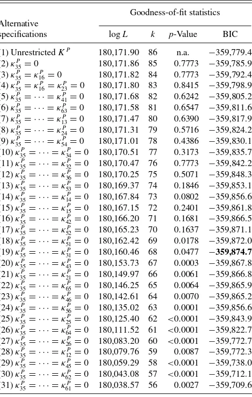
Table 4reports the estimated factor loadings of the state
vari-ables in the corporate bond yield function for each rating cat-egory represented in the data sample. Note that for both U.S. banks and financial firms, lower credit quality tends to imply higher sensitivities to the two common credit risk factors. The exception is the sensitivity of AA-rated U.S. financials to the common credit risk slope factor, which is marginally higher than the value observed for A-rated U.S. financials. Generally speaking, this result implies that the credit spreads of bonds issued by firms with lower credit quality tend to have higher and steeper credit spread curves. Furthermore, we can compare the risk sensitivities for U.S. banks and financial firms. For the benchmark A-rating category, we see that bonds with this rating have nearly identical risk sensitivities across the two sectors. For the AA-rating category, we see greater sensitivities in financial bonds than AA-rated bonds issued by U.S. banks. A partial ex-planation for this difference is the different data sample periods, where yields for AA-rated U.S. banks do not enter the sample
Table 4. Estimated factor loadings in the corporate bond yield functions
Rating αC
0 αLCT α
C
ST α
C
LS α
C SS
U.S. Financials
A 0 −0.0258 −0.0644 1 1
(0.0238) (0.0055)
AA 0.0034 −0.0819 −0.0716 0.9033 1.0400
(0.0002) (0.0212) (0.0062) (0.0058) (0.0113)
U.S. Banks
BBB 0.0002 −0.0333 −0.0732 1.1535 1.0716
(0.0003) (0.0270) (0.0061) (0.0051) (0.0096)
A 0.0000 −0.0326 −0.0564 1.0320 1.0236
(0.0030) (0.0241) (0.0066) (0.0055) (0.0095)
AA −0.0002 −0.0092 −0.0404 0.8239 0.8702
(0.0005) (0.0200) (0.0068) (0.0085) (0.0118)
NOTES: The estimated factor loadings for each of the rating categories for the preferred six-factor model. The data used are weekly, covering the period from January 6, 1995 to July 25, 2008. The numbers in parentheses are the estimated standard deviations of the parameter estimates.
Table 5. Summary statistics for six-factor model-fitted errors
Bank bond yields Financial bond yields Maturity
in months Treasury yields LIBOR rates BBB A AA A AA
Mean
3 −5.52 −0.50 −6.33 −4.36 −3.90 −1.47 0.90
6 −3.53 0.00 3.91 5.18 0.64 3.29 5.08
12 0.27 −0.15 0.18 0.75 1.61 −1.19 0.90
24 2.04 – 1.29 0.05 2.01 −1.30 0.18
36 −0.30 – −1.12 −0.06 1.85 −0.80 −1.31
60 −3.21 – −3.59 −6.36 −9.16 −3.37 −3.98
84 0.49 – 5.14 3.39 7.74 1.43 −1.30
120 12.61 – 0.52 1.37 −0.74 3.30 −0.49
RMSE
3 15.67 10.18 13.28 12.37 11.49 11.66 12.67
6 6.58 0.00 10.15 10.58 11.48 10.15 11.90
12 3.16 8.64 11.58 9.35 11.19 10.72 9.48
24 2.64 – 11.22 7.34 8.50 6.52 7.80
36 1.70 – 12.05 8.94 12.47 8.55 9.57
60 3.91 – 11.58 10.01 13.17 8.88 9.83
84 3.57 – 14.50 9.56 14.87 8.76 8.85
120 14.87 – 14.67 14.15 13.55 12.74 12.83
No. obs. 708 708 708 708 358 708 708
NOTES: This table provides the mean and RMSE of the model-fitted errors in basis points for Treasury bond yields, LIBOR rates, and corporate bond yields for U.S. banks rated BBB, A, and AA and U.S. financial firms rated A and AA. The model used is the preferred six-factor model.
until September 2001. Thus, the previous downturn in the credit cycle is only partially represented for AA-rated banks, while the very calm period from mid-2003 until mid-2007 is fully represented.
Finally,Table 5details the fit of the model for Treasury, bank bond, and LIBOR rates. The fit of the Treasury rates is quite good and only slightly worse than in models of only Treasury yields; see Christensen, Diebold, and Rudebusch (2011), for example. For the corporate bond yields, the root mean squared errors (RMSEs) of the fitted errors are in line with the estimated standard deviation for the fitted errors that we obtain from the Kalman filter, which is estimated atσεc =11.3 basis points.
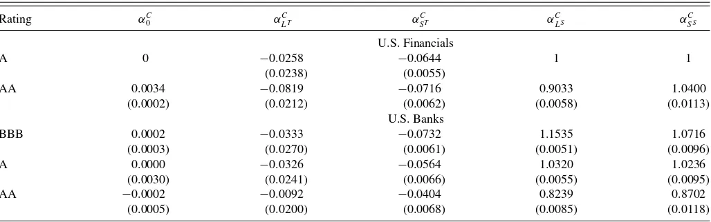
Overall, given the fact that we are fitting a sizeable number of corporate bond yields jointly with only five state variables, the achieved fit of the corporate bond yields appears quite good. The model fits the 6-month LIBOR rate perfectly, while the fit of the other LIBOR rates is well within the range considered acceptable when it comes to regular Treasury bond yield term structure models.Figure 4illustrates the time series of the fitted errors for the 3-month LIBOR rates. Note that there is little deterioration in the model’s ability to fit the LIBOR rates during the financial crisis in 2007 and 2008; thus, the model appears flexible enough to capture the turmoil in the LIBOR market.
4. THE FINANCIAL CRISIS AND CENTRAL BANK ACTIONS
In this section, we use the estimated, reduced-form model to examine the effect on LIBOR rates of the financial crisis and the introduction of the central bank liquidity facilities in December 2007. We also provide supporting evidence and analysis based on the model-implied LIBOR factor.
4.1 Interbank Liquidity Dynamics During the Financial Crisis
Figure 5 focuses on movements in the spread between the
3-month LIBOR rate and the 3-month Treasury yield during the last 18 months of our sample, from the beginning of 2007 through July 25, 2008. There are two key dates during this period. The first, August 9, 2007, marks the start of the tur-moil in many financial markets and the jump in LIBOR rates.
1996 1998 2000 2002 2004 2006 2008
−30
−20
−10
0
10
20
Fitted error in
b
asis points
Figure 4. Fitted model errors of 3-month LIBOR. This figure shows the fitted errors of 3-month LIBOR rates in the six-factor model with the preferred specification ofKP. The data used in the estimation are
from January 6, 1995 to July 25, 2008.
8 0 0 2 7
0 0 2
0
50
100
150
200
Spread in
b
asis points
BNP report Aug. 9
TAF and swap
announcement Dec. 12
Bear Stearns rescue March 24
Figure 5. Spread of 3-month LIBOR over 3-month Treasury yield. This figure shows the spread of the 3-month LIBOR rate over the 3-month Treasury bond yield since the beginning of 2007.
The second, December 12, 2007, marks the announcement by the Federal Reserve and other central banks of a strong new commitment to improve liquidity and the functioning of the in-terbank market. (The Federal Reserve’s initial response to the dislocations in the interbank lending market in the fall of 2007 was to promote and enhance the availability of its discount win-dow as a source of funding. In particular, the Federal Reserve reduced the spread between the discount rate (or primary credit rate) and the target federal funds rate. However, through the end of 2007, discount window borrowing remained relatively low, and interbank lending rates remained quite elevated.) Specifi-cally, the Federal Reserve announced the creation of the TAF, which consisted of periodic auctions of fixed quantities of term funding to sound depository institutions (the first TAF auction occurred on December 17 for $20 billion in 28 day credit and was greatly oversubscribed) and the establishment of coordi-nated dollar liquidity actions with several other central banks. The latter involved reciprocal foreign exchange swap lines, in which dollars were passed through to foreign central banks so they could extend term lending in dollars abroad. The TAF and the swap lines were meant to alleviate the dollar liquidity risk by making cash loans to banks that were secured by those banks’ illiquid but sound assets, and many interpreted the initial mid-December 2007 announcements and actions by central banks as the key events signaling a change in the bank liquidity regime. (Both the TAF and the swap lines were scaled up in size during 2008, and the Federal Reserve subsequently also established several other liquidity facilities that provide loans to financial institutions other than banks, such as the Primary Dealer Credit Facility.) In particular, the initial announcements of the new liq-uidity facilities were accompanied by a widespread realization that the Federal Reserve and other central banks would provide forceful and innovative responses to bank liquidity needs going forward. Therefore, we consider mid-December 2007 as an a priori potential breakpoint in our analysis.
After the central bank announcements and actions in Decem-ber 2007, the LIBOR-treasury spread did fall, but not
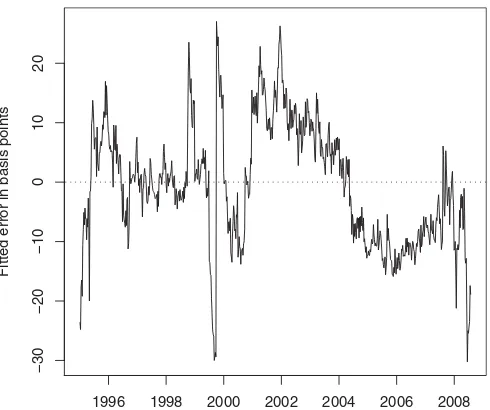
perma-1996 1998 2000 2002 2004 2006 2008
0.045
0.050
0.055
0.060
Val
u
e of Li
b
or−specific factor
Est. mean = 5.61%
TAF and swap announcement Dec. 12, 2007
+/− two st. dev. prior to August 10, 2007
Figure 6. Estimated LIBOR factor from preferred six-factor model. This figure shows the estimated LIBOR-specific factor from the pre-ferred six-factor model. The bond yields and LIBOR rates used in the estimation are weekly data from January 6, 1995 to July 25, 2008.
nently, and it did not revert to its pre-August level. Accordingly, there has been much debate in the literature about the extent to which the central bank liquidity facilities alleviated stress in the interbank market, as noted earlier. We investigate this ques-tion with our estimated model.Figure 6 shows the estimated path of our sixth factor, which is specific to the LIBOR market. Deviations of this factor from its mean (shown by a horizontal dashed line) indicate the direction and approximate size of the difference between the yield on AA-rated U.S. financial bonds and term LIBOR rates of the same maturity. Until December 2007, this factor moved within a fairly close range around its mean. However, following the introduction of the central bank liquidity facilities, it dropped quite low through the end of the sample. The figure appears quite consistent with the presence of a regime change in the dynamic behavior ofXLib
t following
the introduction of the TAF and other central bank liquidity operations.
To statistically test for changes in the dynamic properties of
XtLib, we investigate whether its parameters prior to December 14, 2007, denoted
ψLibpre=κ26P, κ46P, κ56P, κ61P, κ62P, κ64P, κ65P, κ66P, θLibP , σLib, κ
Q
Lib, α Lib
in our preferred specification, changed to a new set of parame-ters, denoted
ψLibpost=κ26P,κ46P,κ56P,κ61P,κ62P,κ64P,κ65P,κ66P,θLibP ,σLib,
κLibQ,αLib.
All other parameters in the model are assumed to remain un-changed. As the Kalman filter can handle time-varying param-eters, we can test this hypothesis using the likelihood ratio test. The estimated dynamic parameters for the non-LIBOR factors in the estimation of our preferred specification with a breakpoint are not meaningfully different from before, as shown inTable 6.
Table 7reports the estimated parameters for the LIBOR-specific
factor and compares them with those for the model without a
Table 6. Parameter estimates for preferred specification with regime switch
KP KP
·,1 K·,P2 K·,P3 K·,P4 K·,P5 θ
P
KP
1,· −1.0719 −1.2081 0 0 0 0.0113 0.0019
(0.1648) (0.2095) (0.0275) (0.0001)
KP
2,· 0.8645 0.5975 0 0 0.1343 −0.0077 0.0020
(0.3724) (0.3965) (0.0580) (0.0239) (0.0002)
KP
3,· 0 0 0.0002 0 0 0.0763 0.0048
(0.0995) (0.1202) (0.0001)
KP
4,· 0 0 1.0340 0.9684 −1.1788 −0.0339 0.0082
(0.5280) (0.1989) (0.1873) (0.0803) (0.0002)
KP
5,· 0 0 0 0 0.8492 −0.0127 0.0264
(0.5465) (0.0525) (0.0007)
NOTES: This table provides the estimated parameters and standard deviations (in parentheses) of theKPmatrix,θPvector, andvolatility matrix for the first five factors in the preferred
joint six-factor model with a regime switch as of December 14, 2007. The data are weekly from January 6, 1995 to July 25, 2008.λTis estimated at 0.6412 (0.0036),λSis estimated at
0.3914 (0.0098). The maximum log-likelihood value is 180,174.56.
breakpoint. The likelihood ratio test of the hypothesis that no breakpoint was observed is
LR=2[180,174.56−180,160.46]=28.2∼χ2(12),
which is highly significant with ap-value of 0.0052. This test suggests that the hypothesis of unchanged parameters can be rejected and that there was a breakpoint during the week before December 14.
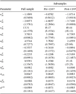
Table 7. Estimated parameters for the LIBOR factor with breakpoint
Subsamples
Parameter Full sample Pre-12/07 Post-12/07
κP
26 −1.1699 −0.8762 −1.8714
(0.5408) (0.6412) (3.0018)
κP
46 −2.8073 −4.8057 −3.7100
(1.3781) (2.2664) (9.0008)
κP
56 13.31 16.17 40.44
(4.1376) (6.1534) (16.12)
κP
61 3.7633 3.1996 0.7395
(0.6882) (0.7795) (4.0891)
κP
62 4.5744 3.7682 2.4559
(0.7277) (0.7997) (25.66)
κP
64 −0.3537 −0.3410 −0.0894
(0.1408) (0.1372) (4.6479)
κP
65 −0.2235 −0.1206 −0.5169
(0.0991) (0.1078) (2.1467)
κP
66 8.9391 8.1580 15.16
(1.3547) (1.5050) (15.25)
θP
Lib 0.0562 0.0562 0.0506
(0.1181) (0.1417) (0.1439)
σLib 0.0047 0.0045 0.0063
(0.0002) (0.0003) (0.0023)
κLibQ 0.0366 0.0373 0.0178
(0.0783) (0.0947) (0.0590)
αLib −0.0569 −0.0571 −0.0565
(0.1181) (0.1417) (0.1440)
NOTES: This table provides the estimated parameters and standard deviations (in parenthe-ses) associated with the LIBOR-specific factor with and without a breakpoint following the establishment of central bank liquidity facilities. The model used is the preferred six-factor model estimated with treasury bond yields and corporate bond yields for U.S. banks and U.S. financial firms in addition to LIBOR rates. The data used are weekly covering the period from January 6, 1995 to July 25, 2008.
To quantify the impact that the introduction of the liquidity facilities had on the interbank market, we use a counterfac-tual analysis of what might have happened had they not been introduced. We use the full-sample model without the break-point to generate a counterfactual path for the 3-month LIBOR rate that suggests what that ratemighthave been if it had been priced in accordance with prevailing conditions in the Trea-sury and corporate bond markets for U.S. financial firms. To quantify this effect, we “turn off” the LIBOR-specific factor by fixing it at its mean prior to December 14, 2007, for the entire sample period, while leaving the remaining factors unchanged at their previously estimated values. Thus, the counterfactual path provides a LIBOR rate consistent with the risk factors re-flected in the yields of bonds issued by AA-rated U.S. financial institutions.
Figure 7illustrates the effect of the counterfactual path on the
3-month LIBOR spread over the 3-month Treasury rate since the beginning of 2007. Note that the model-implied 3 month LIBOR spread is close to the observed spread over this period. Until December 2007, the counterfactual spread was tracking the observed spread relatively closely. However, by the end of 2007, a significant wedge developed between the two. As of the end of our sample on July 25, 2008, the difference between the counterfactual spread and the observed 3-month LIBOR spread was 82 basis points. The counterfactual 3-month LIBOR rate averaged 70 basis points higher than the observed rate from December 2007 through July 2008. (While our analysis dif-fers from that in related studies, our counterfactual result is in line with them. For example, McAndrews, Sarkar, and Wang
(2008)found that the TAF announcement and operations
low-ered the 3-month LIBOR-OIS spread by more than 50 basis points. Wu(2011)also found that the central bank liquidity fa-cilities lowered this spread by 50 to 55 basis points.) Therefore, our empirical results suggest that the announcement of the cen-tral bank liquidity facilities on December 12, 2007 altered the dynamics of the interbank lending market in the intended way, that is, the increased provision of bank liquidity by central banks lowered LIBOR rates relative to where they might have been in the absence of these actions. (Please note that in the absence of a structural model, we cannot explicitly link our results to specific credit events or liquidity services provided.)
8 0 0 2 7
0 0 2
0
50
100
150
200
250
Spread in
b
asis points
BNP report Aug. 9
TAF and swap announcement
Dec. 12
Bear Stearns rescue March 24 LIBOR over Treasury, observed
LIBOR over Treasury, fitted LIBOR over Treasury, counterfactual
Figure 7. Spread of the LIBOR rate over Treasury yield. This figure shows the spread of the observed and fitted 3-month LIBOR rate over the 3-month Treasury bond yield in the preferred six-factor model. The figure also illustrates the spread of the fitted 3-month LIBOR rate when the LIBOR-specific factor is fixed at its historical average prior to December 14, 2007, in effect neutralizing the idiosyncratic effects in the LIBOR market. The illustrated period starts at the beginning of 2007, while the model estimation sample covers the period from January 6, 1995 to July 25, 2008.
4.2 Interpreting the LIBOR Factor
The abnormally large and persistent spread between bank debt yields and LIBOR rates that opened up after mid-December 2007 most likely reflects different liquidity concerns between the lender types in these two markets. The LIBOR rate in the interbank market is based on banks providing other banks with short-term funding. In contrast, the bank bond rates are derived from debt obligations issued to a broader class of investors that mainly consists of nonbank institutions. While these two types of lenders most likely attach similar default probabilities and prices to credit risk, they likely have different tolerances for liquidity risk. The different degrees to which central bank liquidity operations lowered liquidity concerns in the interbank market by more than in the bank bond market should be observed in the spread between these two market yields and is captured in the model-implied LIBOR factor.
There are two other explanations that could account for the increased spread between bank debt yields and LIBOR rates. The first explanation centers on changes in the quality of the data. Starting in April 2008, reports circulated that the banks in the LIBOR panel for U.S. dollar-denominated term deposits were underreporting their actual borrowing costs. This under-reporting would suggest that distress in the interbank market was more severe than reflected in the observed LIBOR rates. The persistence of the high LIBOR spread through the end of our sample period lessens the effect of these concerns for our study, but remains present within our modeling framework. Al-ternatively, the quality of the corporate bond data, especially since August 2007, could be questioned due perhaps to reduced bond trading. Again, the persistence of the larger spread over
several months weakens this possible explanation, but cannot completely dispel it.
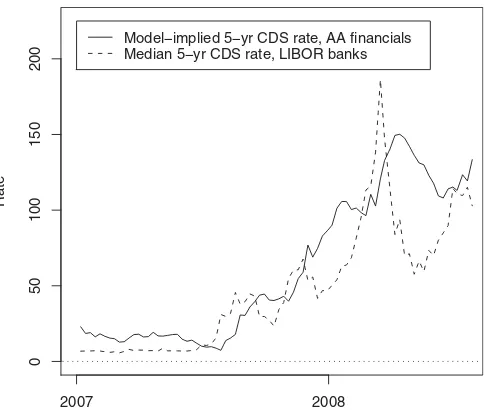
Aside from data quality, the second alternative explanation for the larger spread is the possibility of a change in the relative credit risk characteristics between the bank debt and interbank loan markets; for example, through changes in perceived recov-ery rates. (An unsecured deposit (e.g., an interbank loan) is more senior in the liability structure of a bank than senior unsecured debt. McAndrews, Sarkar, and Wang(2008)mentioned a recov-ery rate of 91.25% for unsecured deposits at banks with assets larger than $5 billion, as per the work of Kuritzkes, Schuer-mann, and Weiner(2005). On the other hand, the data provider Markit typically works with a recovery rate as low as 40% in its pricing of credit default swap contracts. However, it is not clear why this difference in recovery rates would have changed dra-matically in December 2007.) During our sample and notably even during the 2001 recession, there were no substantial differ-ences in relative credit risk between the two markets. However, changes could have occurred in the relative credit risk between the LIBOR panel of international, AA-rated banks, and the do-mestic AA-rated banks and financial firms used to construct the Bloomberg corporate yield curves. To examine this possibility within the context of our model, we generated synthetic 5-year CDS rates for the U.S. AA-rated financial firms and compared these with the median 5-year CDS rate for the banks in the LI-BOR panel. CDS rates are readily calculated from our model using the instantaneous credit spread for AA-rated U.S. finan-cial firms, as presented earlier, and a recovery rate assumption of 50%; see Appendix B for further details.Figure 8presents these model-implied 5-year CDS rates relative to the median of the
8 0 0 2 7
0 0 2
0
5
0
100
150
200
Rate
Model−implied 5−yr CDS rate, AA financials Median 5−yr CDS rate, LIBOR banks
Figure 8. Model-generated CDS spreads. This figure shows the implied 5-year CDS rates for AA-rated U.S. financial firms based on the estimated parameters and factor paths from the preferred six-factor LIBOR model. The median of the 5-year CDS rates of the 16 LIBOR panel banks on each observation date is shown. To align the level of the model-implied estimates with the observed CDS rates, the difference between the 5-year Treasury par bond yield and the 5-year swap rate has been added. The illustrated period starts at the beginning of 2007, while the model estimation sample covers the period from January 6, 1995 to July 25, 2008.
2007 2008 2009 2010 2011
−400
−300
−200
−100
0
100
2007 2008 2009 2010 2011
−400
−300
−200
−100
0
100
Diff
erence in
b
asis points
TAF in operation BNP
report
Bear Stearns
rescue
Lehman Brothers
bankruptcy <===
FOMC 12/08
Figure 9. Deviation of estimated LIBOR factor from its pre-TAF average for the 2007–2010 period. This figure shows the deviation of the model-implied LIBOR factor from its pre-TAF average based on the preferred specification of the six-factor model for the period from January 6, 2007 to December 31, 2010. The shaded region highlights the period over which TAF auctions occurred.
corresponding observed CDS rates for the banks in the LIBOR panel. The series have a correlation of nearly 90% in levels, suggesting that the underlying credit dynamics for AA-rated financial institutions estimated by our model are very similar to those observed in the CDS market. This result supports our assumption of common credit characteristics across the LIBOR and bank debt panels and our view that this relationship did not materially change around the announcement of the central bank liquidity facilities.
To expand the analysis of the model-implied LIBOR factor beyond the defined sample period, we extend the sample up through year-end 2010.Figure 9presents the deviation of the estimated LIBOR factor from its pre-TAF average based on weekly data from January 1995 through December 2010, al-though without the structural break discussed previously. This extended sample encompasses the wave of financial defaults in September 2008, the setting of the Federal Reserver’s policy rate to zero, and the introduction of unconventional monetary policy actions. All of these events and policy responses affected the liquidity dynamics of the interbank market differently than the wider bank debt market, and the deviation of the LIBOR factor from its pre-TAF average provides a summary measure of those effects. For example, during the period from September 2008 with the failure of Lehman Brothers to the December 2008 FOMC at which the policy rate was lowered to zero and various unconventional monetary policy actions were introduced, the LIBOR factor dropped precipitously in light of the near-collapse of important components of the financial system, which caused the yields on bank debt to spike up dramatically relative to the rates in the interbank market that varied less thanks to the policy initiatives. The condition of both markets improved gradually during the course of 2009 as a variety of government programs, such as the FDIC’s Temporary Liquidity Guarantee Program
(TLGP), and additional Federal Reserve liquidity facilities took effect. By the end of 2009, market conditions had improved sufficiently that the Federal Reserve announced the termination of the TAF auctions as well as other liquidity facilities at the January 2010 FOMC meeting. The LIBOR factor closely tracks these market developments and returned to its pre-TAF average level by October 2009 and remained there through the end of the sample in December 2010. This analysis provides further support for the model’s ability to capture the reduced-form liq-uidity dynamics of the interbank market relative to the wider market for bank debt.
5. CONCLUSION
In this article, we address the question of whether interbank lending rates have responded to central bank liquidity operations by using a six-factor AFNS model that encompasses Treasury yields, financial corporate debt yields, and LIBOR rates. Our results provide support for the view that these operations low-ered LIBOR rates starting in December 2007 and through the end of our sample in July 2008. We find that the parameters governing the LIBOR factor in our model appear to change after the introduction of the liquidity facilities, that is, the hy-pothesis of constant parameters over the full sample period is rejected. This result suggests that the behavior of this factor, and thus of the LIBOR market, was directly affected by these central bank liquidity operations. To quantify this effect, we use the model to construct a counterfactual path for the 3-month LIBOR rate. The counterfactual 3-month LIBOR rate averaged significantly higher than the observed rate from December 2007 into midyear 2008, which suggests that if the central bank liq-uidity operations had not occurred, the 3-month LIBOR spread over Treasuries would have been even higher than the observed historical spread.
APPENDIX A: CONVERSION OF INTEREST RATE DATA
The Bloomberg fair-value, zero-coupon yield curves are gen-erated for particular (sector,rating) segments of the corporate bond market using individual bond prices, both indicative and executable, as quoted by price contributors over a specified time window. Based on these bond datasets, option-adjusted spreads are generated, and these adjusted bond yields are converted into zero-coupon yield curves using piecewise linear functions.
We convert the Bloomberg data for financial corporate bond rates into continuously compounded yields. Then-year yield at timet,rt(n), the corresponding zero-coupon bond price,Pt(n),
and the continuously compounded yield,yt(n), are related by
Pt(n)=
1 (1+rt(n))n
=e−yt(n)n ⇐⇒
yt(n)= −
1
nln
1 (1+rt(n))n
=ln(1+rt(n)).
For maturities shorter than 1 year, we assume the standard con-vention of linear interest rates. For example, the zero-coupon