TERRESTRIAL LASER SCANNING FOR GEOMETRY EXTRACTION AND CHANGE
MONITORING OF RUBBLE MOUND BREAKWATERS
I. Puente a, *, R. Lindenberghb, H. González-Jorge a, P. Arias a
a Dept. of Natural Resources and Environmental Engineering, University of Vigo, Maxwell s/n, 36310, Vigo, Spain -
(ipuente, higiniog, parias)@uvigo.es
b Dept. of Geoscience and Remote Sensing, Delft University of Technology, Stevinweg 1, 2628 CN, Delft, The
Netherlands – [email protected]
Commission V, WG V/3
KEY WORDS: LiDAR, point cloud, segmentation, breakwater modeling, change detection
ABSTRACT:
Rubble mound breakwaters are coastal defense structures that protect harbors and beaches from the impacts of both littoral drift and storm waves. They occasionally break, leading to catastrophic damage to surrounding human populations and resulting in huge economic and environmental losses. Ensuring their stability is considered to be of vital importance and the major reason for setting up breakwater monitoring systems. Terrestrial laser scanning has been recognized as a monitoring technique of existing infrastructures. Its capability for measuring large amounts of accurate points in a short period of time is also well proven. In this paper we first introduce a method for the automatic extraction of face geometry of concrete cubic blocks, as typically used in breakwaters. Point clouds are segmented based on their orientation and location. Then we compare corresponding cuboids of three co-registered point clouds to estimate their transformation parameters over time. The first method is demonstrated on scan data from the Baiona breakwater (Spain) while the change detection is demonstrated on repeated scan data of concrete bricks, where the changing scenario was simulated. The application of the presented methodology has verified its effectiveness for outlining the 3D breakwater units and analyzing their changes at the millimeter level. Breakwater management activities could benefit from this initial version of the method in order to improve their productivity.
* Corresponding author.
1. INTRODUCTION
Structural monitoring has become nowadays an important research area involved in the structural integrity assessment of civil infrastructures. Engineering communities have shown an increasing interest to monitor bridges (Enckell et al., 2011; Ye et al., 2013), tunnels (Lindenbergh et al., 2005; Puente et al., 2014; Sharma et al., 2001) and other structures (Valença et al., 2013) and to detect damage at the earliest stages. Specifically, rubble mound breakwaters (Corredor et al., 2013) are commonly employed to protect important coastal areas such as ports, marinas or beaches from the effects of attacking ocean waves.
Some studies have described fairly extensively the fluid-structure interaction (Altomare et al., 2014) and the breakwater monitoring (Del Grosso et al., 2003; Yoon et al., 2012). It is crucial to detect local defects on time, such as displacements, breakage or removals of the concrete armor units (CAUs), before they become a real threat to the safety of breakwaters. The observed damages in these structures can be divided into sliding, settlement or toppling, directly causing displacements, breakage or removals of the concrete armor units. Other defects such as scouring at dike foundations can also occurr and tend to propagate into more serious damages under extreme wave forces. Therefore, it is advantageous to develop a methodology which identifies local movements in these coastal defense structures.
Detection of changes using LiDAR data is growing quickly in many engineering applications (Lindenbergh, 2010; Monserrat
and Crosetto, 2008). This technology allows for low risk and rapid collection of accurate geospatial information as an alternative for traditional surveying techniques. It has been proved that an easy procedure to map and monitor topographic changes is by using repeated LiDAR measurements from a fixed position (Van Goor et al., 2011) or any mobile platform (Puente et al., 2013).
This work presents a novel approach to automatically evaluate changes in rubble mound breakwaters using point clouds of different epochs. The method first identifies single segments from each armour unit and their face geometry is outlined. Secondly, the algorithm looks for corresponding cuboids in different epochs and estimates their rigid body transformation parameters. The paper has been organized into four main sections. The second reflects the formal description of the algorithm. In section three, the results are presented and discussed. Finally, some conclusions are provided.
2. METHODOLOGY
In this section, we focus on the identification of individual planar segments representing the cuboid faces. Those segments are later grouped together to form individual cuboids (or breakwater units), which are used to monitor changes in the structure.
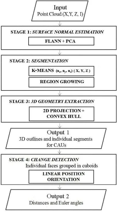
The algorithm overview summarizes the following steps, as shown in Figure 1.
Figure 1. Algorithm overview for 3D outlines of the CAUs
2.1 Surface normal estimation
The raw point cloud data is originally represented by the 3D Cartesian coordinates and the intensity value (X, Y, Z, I). We use the location of the laser scanner as the origin of each scan’s local coordinate system. However, the segmentation procedure described in Section 2.2 will require surface normal estimates as a prerequisite. We first determine the local neighbors of each point p in point cloud. There are several nearest neighbor methods available, such as K-Nearest Neighbours search (KNNsearch), Approximate Nearest Neighbour (ANN) or its variant FLANN (Fast Library for Approximate Nearest Neighbour), each of them implementing a number of different search strategies and data structures, based on kd-trees and box-decomposition trees. For this case study, we used FLANN (Muja and Lowe, 2009), written in C++ but with binding for the Matlab language.
The estimated surface normal for the point p is then the normal n = (nx, ny, nz) to the plane that best fits the neighboring data points in the least square sense. This plane is determined using Principal Component Analysis (PCA).The approximate surface normal, oriented outwards, is then the eigenvector associated with the smallest eigenvalue of the symmetric positive semi-definite variance-covariance matrix of the neighboring data points (Castillo and Zhao, 2009). The authors will check if the cuboid surface normals have a positive orientation, that is, pointing towards the exterior of the surface, using the scanning direction and the dot product of both vectors.
It should be noted that in general, computing the local neighborhood represents the main computational cost associated with surface normal estimation.
2.2 Segmentation
The resulting values of the PCA are used to reshape the original data matrix (X, Y, Z, I) into a new one, where each point of the cloud will now have 9 data values: X, Y, Z coordinates plus 3 surface normal coordinates (nx, ny, nz) and γ eigenvalues (λ1, λ2, λ3). Before the segmentation process starts, we first filter the
dataset based on the third eigenvalue (λ3). Raw data points with
a greater λ3 will be filtered out, as they mostly correspond to edges or noise.
In the following step, we select a clustering method for grouping the previously filtered data based on their surface normal orientations. There are two common approaches: hierarchical clustering and k-means algorithm. For this case study, we used the latter. K-means clustering treats each observation ni = (nxi, nyi, nzi) as an object having a location in space. If the set N={ n1, …, ni} defines the i points to be clustered, we seek a collection of k mutually exclusive subsets of N, say, C1,….Ck, that minimizes the sum of distances from each point to its cluster centroid, over all clusters. Distances are measured using the squared Euclidean distance metric and the process is reiterated until the clustering processes stabilize, which basically means that no points swap cluster anymore (Spath, 1985).
This method needs both k and the initial centroid positions (also known as seeds) to be specified to initialize it (Chiang and Mirkin, 2010). For the case study, we selected the seeds from N at random while the right number of clusters k was estimated by plotting all normal directions on a stereographic projection. Then, by applying some image processing techniques with Matlab, k is semi-automatically estimated. Intermediate steps include the image binarization, and the centroid and area computation for each cluster in the binary image. In fact, the only parameter provided by the user is the minimum number of pixels that compose each cluster area.
It is therefore possible to segment point clouds into subsets, each one made of points with similar orientation. Then, for each cluster Ck, we applied a k-means clustering for the second time where the input data matrix is composed of X, Y, Z coordinates. We use an over-segmentation approach in some clusters but in this way, we assure one single segment per cluster and also, we can delete those small and unrepresentative clusters, classifying them as outliers. used specifies the maximum acceptable angle between the normal of the current seed and its neighbors. The latter are computed by searching all the centroids that are within distance dp of the current seed.
2.3 Automatic geometry extraction
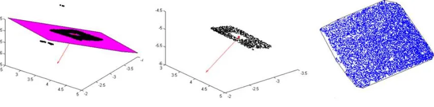
When we process the clustered laser scanning data, we still need to remove some noisy points that clearly do not belong to a cube face (see Figure 2). To overcome this problem, we adjust a plane to each cluster, defined by the mean normal vector and its
Figure 2. Filtering of a noisy planar segment and resultant 2D convex hull
centroid. The orthogonal distance from each cluster point, d, to the plane is then computed and a threshold value (dt) is chosen
by the user to remove those noisy points.
The reduction of each cluster into 2D using the previously defined plane is the next step. Then, we apply a convex hull algorithm (Preparata and Hong, 1977) in order to create the bounding polygon for each cluster. Finally, we convert the 2D polygons into 3D outlines of the cube faces.
2.4 Identifying changes in concrete units
The next step after the 3D outlining and segmentation processes is to identify possible changes in the breakwater armor units that could appear with time. In quasi-time-invariant environments, when a breakwater is scanned twice from the same scan position and under the same conditions, the segmentation results should be similar. Therefore, a segment in one scan that has no counterpart in the second scan would indicate a possible change.
In practice, to monitor all the breakwater units along time, corresponding block pairs among epochs will be manually matched, as there is no intrinsic correspondence between segments based just on distance, size or orientation. To achieve the objective, a validation experiment is designed in which bricks with alphanumeric characters on their faces are considered (see Figure 4).
First of all, all planar faces identified for each epoch are connected to represent individual rigid blocks. That is, an automatic algorithm recursively matches three or more corresponding faces of the same block.This procedure can be reached again through a region growing algorithm that clusters the faces based on a distance threshold (dmax) and the relationship between the convexities of connected segments. Every planar segment is defined by its normal vector n and the centroid of the points in the segment.If the intersection of the lines defined by the normal vector and centroid from two adjacent faces, lies within the block, both faces are grouped together. Otherwise, they are not grouped. Once the cuboids are individually identified for each epoch, the comparison is straightforward. We denote the set of all cuboids from the first epoch as CI and the set of all cuboids from the second epoch as CII. Cuboid 1 from epoch I is notated as CI1 while the same cuboid from epoch II is notated as CII1.
In order to parameterize the location in 3D space, the centers of gravity and the Euler angles of the cuboids are computed. Euler angles are three angles used to represent the orientation of a rigid body relative to a coordinate system. For the sake of simplicity, we consider here the case of just one cuboid C1, monitored in epochs I, II and III. The method would be then extended in the same way to the rest of cuboids.
We can define the centroid of the cuboid as the intersection of the lines formed by the normal vector and the centroid of each face forming the cuboid. The same orthogonal vectors are used to calculate the orientation of the cuboid in a fixed reference frame (which is the scanner coordinate system). The three resulting angles (α, , ) are computed as the dot product between each face normal unit vector n and its corresponding fixed axis (u, v, w) following the right-hand rule.
The Cartesian coordinates of both centers of gravity from CI1 and CII1 are used to determine the Euclidean distance (Equation 1) and the translations tx, ty and tz along x, y and z- axes,
respectively. Monitoring the rotations can be easily achieved by looking at the Euler angles and comparing them with the fixed coordinate system.
(1)
3. RESULTS AND DISCUSSION
In this section, the methodology explained in section 2 is illustrated for two case studies. The 3D geometry extraction is demonstrated on armor units in a rubble mound breakwater. The change detection procedure was tested with a validation experiment of three cuboids where the scenario was simulated.
3.1 Data description
Baiona breakwater is the main defensive structure around the Port of Baiona, in northwestern Spain (Figure 3b). It is an old rubble mound breakwater with conventional concrete cubes as armor units. For testing the geometry extraction algorithm, authors selected an area of 14 x 5.5 m (Figure 3a), sampled by approximately 230 thousand points scanned with a Faro Focus 3D (Faro, 2013a). This is a phase-based system, whose measurements are taken continuously. This fact makes it suitable for precise surveys.
Figure 3. Baiona breakwater
For the change monitoring task, we considered concrete bricks (Figure 4) that were rotated and translated in a controlled manner during three consecutive epochs. The presented scenario was designed to be realistic under higher-than-design storm conditions, where concrete armors resist with only a few units being extracted from the breakwater. But generally, breakwater units will undergo very small dislocations.
Individual scans were performed from the same scan position using the Faro Photon 120 phase-based scanner (Faro, 2013b). As a consequence, point clouds were already registered in a common coordinate system and no control points were required.
Figure 4. Three concrete bricks employed in the validation experiment for change monitoring: (a, c) Epoch I; (b, d) Epoch
III
3.2 Surface normal estimation and segmentation
The choice of the number of neighbors, s, is essential for the quality of the calculated normal. Low s values are sensitive to noise, while higher values may compensate the noise problem but also increase the processing time. Thus, PCA was performed using the 50 closest points of each point in the point cloud (Belton and Lichti, 2006).
The point cloud from Figure 3a was segmented into planar patches after k-means clustering. The parameter value k=25 was first estimated by plotting all cluster orientations on a stereographic projection (Figure 5).This resulted in 25 segments for the first round k-means and in 125 segments for the second round k-means (Figure 6a).
Figure 5. Stereoplot of all the orientations of the concrete armor faces in the 3D model
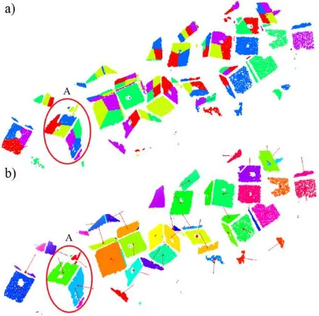
Over-segmented patches were then clustered into cube faces using the region growing method described in detail in Section 2.2. Here, the parameter values, αp = 20◦ and dp = 0.9 m were used. This setting resulted in 47 planar segments (Figure 6b). For example, in the following cube marked by a capital ‘A’, three segments in red, blue and yellow were grouped in one resulting green colored face while the set of purple, green and dark blue segments resulted in one cyan cube face. The other
three segments remain unclustered as they don’t fulfill the
conditions specified in the method. In fact, this approach requires both parameters to be defined precisely in order to succeed. On the contrary, nearly-parallel adjacent segments from different cubes but with the same normal orientation, could be wrongly group together.
Figure 6. (a) Over segmentation of cube faces. (b) Segmented cube faces after Region Growing with their normal vector
representation.
Figure 7. 3D outlines of the cube faces
Figure 7 shows the 3D outlines after the 2D reduction of the previously segmented cube faces and the convex hull implementation.
3.3 Change monitoring in cuboids
The workflow explained in Sections 2.1-2.3 was again applied to this dataset composed of three concrete bricks. The value k=4
Figure 8. Top view of the cuboids 1, 2 and 3 (from left to right) studied in three different epochs. The faces are not grouped in cuboids at this point.
Figure 9. Identification of cuboids in epoch 1. The faces are now grouped.
was used in the first k-means clustering. In Figure 8, every planar segment was identified and plotted in random color. The concrete bricks were modeled as cuboids, where each pair of adjacent faces or segments meets in a right angle. This process was achieved using the region growing algorithm described in Section 2.4. Two parameters were required: a distance threshold (dmax =0.010 m) and the relationship between the convexities of connected segments. Figure 9 illustrates the results from this step for CI.
In order to define their placement in 3D, the linear position and orientation of the cuboids were computed. Typically, the reference point chosen is coincident with the centroid of the rigid body. The cuboid orientation is given by its three orthogonal vectors.
In the following, the centers of gravity of each cuboid and its Euler angles were derived. The results only consider the case of just one cuboid C1, monitored in epochs I, II and III. However, the procedure can be applied to the whole set of corresponding cuboid pairs identified by the user.
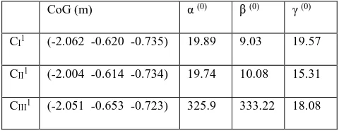
Table 1. Centers of Gravity and Euler angles for CI1, CII1, CIII1. Changes were manually applied to the cuboids.
CoG (m) α (0) (0) (0)
CI1 (-2.062 -0.620 -0.735) 19.89 9.03 19.57
CII1 (-2.004 -0.614 -0.734) 19.74 10.08 15.31
CIII1 (-2.051 -0.653 -0.723) 325.9 333.22 18.08
Therefore, it is now possible to determine the distances between centers of gravity of cuboids and the orientation (or relative orientation) with time. For example, the displacement relative to epoch I is dCI1CII1 = 0.058 m and the translations along the axis for CII1 are tx = 0.058 m, ty= 0.006 m and tz= 0.001 m. The
distance traveled for CIII1 with reference to epoch II is dCII1CIII1 = 0.062 m with tx = -0.047 m, ty = -0.039 m and tz= 0.011 m.
Although there is no ground truth available for the resulting values in Table 1, they are as expected: in epoch II, the C1 transformation consists of only a translation, so the Euler angles remain almost identical. In epoch III, C1 rotated mainly around the z and x axes and it was also translated (see Figure 8).
The method presented here is an initial version using data acquired from a single scan position. It could be extended to larger breakwaters, though multiple scans from different standpoints in one epoch would be needed. In that case, datasets should be registered with a high accuracy using reflective targets (control points) placed on the scene. The result would be one point cloud per epoch. Moreover, occlusions would be mostly solved, when parts of the breakwater surface that were not visible from one scan position would be captured by another one.
4. CONCLUSIONS
In this paper a new methodology has been presented for the 3D outline of concrete armor units in a breakwater and the monitoring of their displacements and rotations. In an efficient manner, the original point cloud is segmented into planar patches that can be identified over time (after the manual marking of corresponding segments and cuboids). This method later compares two or more matched cuboids in different epochs, letting the user to monitor their 3D placement over time. This fact makes this method useful to detect local defects at early stages, avoiding them to affect the structural stability of the breakwaters.
The method is computationally efficient and it can be easily adapted to other fields of application where block-like structures must be identified and tracked along time.
The best segmentation parameters vary within a scene, depending on the objects present. However, some improvements can be made to enhance the segmentation process. These are linked to the varying point cloud quality (such as areas with lower point density or higher incident angles), plane fitting errors or measurement errors that will definitely affect the aforementioned process.
Other challenges are related to occlusions, that could prevent the monitoring of corresponding cuboids or the edge effect that results in noisy points that interfere negatively in the particle hydrodynamics. Computers and Structures, 130, pp. 34-45.
Belton, D. and Lichti, D., 2006. Classification and segmentation of terrestrial laser scanner point clouds using local variance information, ISPRS Journal of Photogrammetry and Remote sensing, 36(5), pp. 44-49.
Castillo, E. and Zhao, H., 2009. Point cloud segmentation via constrained non linear least squares surface normal estimates, Recent UCLA Computational and Applied Mathematics Reports.
Chiang, M.M.-T and Mirkin, B., 2010. Intelligent choice of the number of clusters in k-means clustering: An experimental study with different cluster spreads. Journal of Classification, 27 (1), pp. 3-40.
Corredor, A., Santos, M., Peña, E., Maciñeira, E., Gómez.Martín, M.E., and Medina, J., 2013.Designing and Constructing Cubipod Armored Breakwaters in the Ports of Malaga and Punta Langosteira (Spain). In: Proceedings of the ICE Coasts, Marine Structures and Breakwaters conference, Edinburgh, Scotland http://www.ice-conferences.com/ICE-Breakwaters (17 Feb. 2014).
Del Grosso, A., Lanata, F., Inaudi, D., Posenato, D. and Pieracci, A., 2003. Breakwater deformation monitoring by automatic and remote GPS system. In: Proceedings of the 1st
International Conference on Structural Health Monitoring and Intelligent Infrastructure, Tokyo, Japan, pp. 369-376.
Enckell, M., Glisic, B., Myrvoll, F. and Bergstrand, B., 2011. Evaluation of a large-scale bridge strain, temperature and crack monitoring with distributed fibre optic sensors. Journal of Civil Structural Health Monitoring, 1(1-2), pp.37-46.
Lindenbergh, R.C., 2010. Engineering Applications. In G. Vosselman and H.-G. Maas (Eds.), Airborne and Terrestrial Laser Scanning. Whittles Publishing, Dunbeath, Scotland, pp. 237-242.
Monserrat, O. and Crosetto, M., 2008. Deformation measurement using terrestrial laser scanning data and least squares 3D surface matching. ISPRS Journal of Photogrammetry and Remote Sensing, 63(1), pp.142-154.
Muja, M. and Lowe, David G., 2009. Fast Approximate Nearest Neighbors with Automatic Algorithm Configuration. In: Proceedings of the VISAAP International Conference on Computer Vision Theory and Applications,Lisbon, Portugal, pp.331-340.
Preparata, F.P. and Hong, S.J., 1977. Convex hulls of finite sets of points in two and three dimensions. Communications of the Association for Computing Machinery, 20(2), pp. 87–93.
Puente, I., Solla, M., González-Jorge, H. and Arias, P., 2013. Validation of LiDAR surveying for measuring pavement layer thicknesses and volumes. NDT & E International, 60, pp. 70-Segmentation of point clouds using smoothness constraint. In: The International Archives of the Photogrammetry, Remote Sensing and Spatial Information Sciences, Dresden, Germany, Vol. XXXVI, Part 5, pp. 248-253.
Sharma, J.S., Hefny, A.M., Zhao, J., and Chan, C.W., 2001. Effect of large excavation on deformation of adjacent MRT tunnels. Tunnelling and Underground Space Technology, 16(2), pp.93-98.
Spath, H., 1985. Cluster Dissection and Analysis: Theory, FORTRAN Programs, Examples. Translated by J. Goldschmidt. New York: Halsted Press.
Valença, J., Días-da-Costa, Gonçalves, L., Júlio, E., and Araújo, H., 2013. Automatic concrete health monitoring: assessment and monitoring of concrete surfaces. Structure and infrastructure engineering, In press. DOI: 10.1080/15732479.2013.835326.
Van Goor, B., Lindenbergh, R., and Soudarissanane, S., 2011. Identifying corresponding segments from repeated scan data. In: The International Archives of the Photogrammetry, Remote Sensing and Spatial Information Sciences, Calgary, Canada, Vol. XXXVIII-5/W12, pp.295-300.
Ye, X.W., Ni, Y.Q., Wong, K.Y. and Ko, J.M., 2012. Statistical analysis of stress spectra for fatigue life assessment of steel bridges with structural health monitoring data. Engineering Structures, 45, pp.166-176.
Yoon, H.-S., Lee, S.-Y., Kim, J.-T. and Yi, J.-H. 2012. Field implementation of wireless vibration sensing system for monitoring of harbor caisson breakwaters. International Journal of Distributed Sensor Networks, art. No. 597546.
ACKNOWLEDGEMENTS
Authors want to give thanks to the Spanish Ministry of Economy and Competitiveness and Xunta de Galicia for the
financial support given; Human Resources programs BES-2010-034106 and IPP055-EXP44 and Projects Code No. EM2015/005 and IN852A2013/29.