Ken Kleinman and Nicholas J. Horton
Kleinman and Horton
Data Management,
Statistical Analysis,
and Graphics
S E C O N D E D I T I O N
SAS
and
Data Management,
Statistical Analysis,
and Graphics
S E C O N D E D I T I O N
Ken Kleinman
Department of Population Medicine
Harvard Medical School and
Harvard Pilgrim Health Care Institute
Boston, Massachusetts, U.S.A.
Nicholas J. Horton
Department of Mathematics and Statistics
Amherst College
Amherst, Massachusetts, U.S.A.
SAS
and
© 2014 by Taylor & Francis Group, LLC
CRC Press is an imprint of Taylor & Francis Group, an Informa business
No claim to original U.S. Government works Version Date: 20140415
International Standard Book Number-13: 978-1-4665-8450-1 (eBook - PDF)
This book contains information obtained from authentic and highly regarded sources. Reasonable efforts have been made to publish reliable data and information, but the author and publisher cannot assume responsibility for the validity of all materials or the consequences of their use. The authors and publishers have attempted to trace the copyright holders of all material repro-duced in this publication and apologize to copyright holders if permission to publish in this form has not been obtained. If any copyright material has not been acknowledged please write and let us know so we may rectify in any future reprint.
Except as permitted under U.S. Copyright Law, no part of this book may be reprinted, reproduced, transmitted, or utilized in any form by any electronic, mechanical, or other means, now known or hereafter invented, including photocopying, microfilming, and recording, or in any information storage or retrieval system, without written permission from the publishers.
For permission to photocopy or use material electronically from this work, please access www.copyright.com (http://www.copy-right.com/) or contact the Copyright Clearance Center, Inc. (CCC), 222 Rosewood Drive, Danvers, MA 01923, 978-750-8400. CCC is a not-for-profit organization that provides licenses and registration for a variety of users. For organizations that have been granted a photocopy license by the CCC, a separate system of payment has been arranged.
Trademark Notice: Product or corporate names may be trademarks or registered trademarks, and are used only for identifica-tion and explanaidentifica-tion without intent to infringe.
Contents
List of figures xvii
List of tables xix
Preface to the second edition xxi
Preface to the first edition xxiii
1 Data input and output 1
1.1 Input . . . 1
1.1.1 Native dataset . . . 1
1.1.2 Fixed format text files . . . 2
1.1.3 Other fixed files . . . 3
1.1.4 Reading more complex text files . . . 3
1.1.5 Comma separated value (CSV) files . . . 4
1.1.6 Read sheets from an Excel file . . . 5
1.1.7 Read data from R into SAS . . . 5
1.1.8 Read data from SAS into R . . . 6
1.1.9 Reading datasets in other formats . . . 6
1.1.10 Reading data with a variable number of words in a field . . . 7
1.1.11 Read a file byte by byte . . . 8
1.1.12 Access data from a URL . . . 9
1.1.13 Read an XML-formatted file . . . 9
1.1.14 Manual data entry . . . 10
1.2 Output . . . 11
1.2.1 Displaying data . . . 11
1.2.2 Number of digits to display . . . 11
1.2.3 Save a native dataset . . . 12
1.2.4 Creating datasets in text format . . . 12
1.2.5 Creating Excel spreadsheets . . . 12
1.2.6 Creating files for use by other packages . . . 13
1.2.7 Creating HTML formatted output . . . 14
1.2.8 Creating XML datasets and output . . . 14
1.3 Further resources . . . 15
2 Data management 17 2.1 Structure and meta-data . . . 17
2.1.1 Access variables from a dataset . . . 17
2.1.2 Names of variables and their types . . . 17
vi CONTENTS
2.1.4 Label variables . . . 18
2.1.5 Add comment to a dataset or variable . . . 19
2.2 Derived variables and data manipulation . . . 19
2.2.1 Add derived variable to a dataset . . . 19
2.2.2 Rename variables in a dataset . . . 19
2.2.3 Create string variables from numeric variables . . . 20
2.2.4 Create categorical variables from continuous variables . . . 20
2.2.5 Recode a categorical variable . . . 21
2.2.6 Create a categorical variable using logic . . . 21
2.2.7 Create numeric variables from string variables . . . 22
2.2.8 Extract characters from string variables . . . 23
2.2.9 Length of string variables . . . 23
2.2.10 Concatenate string variables . . . 24
2.2.11 Set operations . . . 24
2.2.12 Find strings within string variables . . . 25
2.2.13 Find approximate strings . . . 25
2.2.14 Replace strings within string variables . . . 26
2.2.15 Split strings into multiple strings . . . 26
2.2.16 Remove spaces around string variables . . . 27
2.2.17 Upper to lower case . . . 27
2.2.18 Lagged variable . . . 28
2.2.19 Formatting values of variables . . . 28
2.2.20 Perl interface . . . 29
2.2.21 Accessing databases using SQL (structured query language) . . . . 29
2.3 Merging, combining, and subsetting datasets . . . 29
2.3.1 Subsetting observations . . . 30
2.3.2 Drop or keep variables in a dataset . . . 30
2.3.3 Random sample of a dataset . . . 31
2.3.4 Observation number . . . 32
2.3.5 Keep unique values . . . 32
2.3.6 Identify duplicated values . . . 32
2.3.7 Convert from wide to long (tall) format . . . 33
2.3.8 Convert from long (tall) to wide format . . . 34
2.3.9 Concatenate and stack datasets . . . 35
2.3.10 Sort datasets . . . 35
2.3.11 Merge datasets . . . 35
2.4 Date and time variables . . . 37
2.4.1 Create date variable . . . 37
2.4.2 Extract weekday . . . 38
2.4.3 Extract month . . . 38
2.4.4 Extract year . . . 38
2.4.5 Extract quarter . . . 38
2.4.6 Create time variable . . . 39
2.5 Further resources . . . 39
2.6 Examples . . . 39
2.6.1 Data input and output . . . 39
2.6.2 Data display . . . 43
2.6.3 Derived variables and data manipulation . . . 44
CONTENTS vii
3 Statistical and mathematical functions 53
3.1 Probability distributions and random number generation . . . 53
3.1.1 Probability density function . . . 53
3.1.2 Quantiles of a probability density function . . . 54
3.1.3 Setting the random number seed . . . 55
3.1.4 Uniform random variables . . . 55
3.1.5 Multinomial random variables . . . 56
3.1.6 Normal random variables . . . 56
3.1.7 Multivariate normal random variables . . . 56
3.1.8 Truncated multivariate normal random variables . . . 58
3.1.9 Exponential random variables . . . 58
3.1.10 Other random variables . . . 58
3.2 Mathematical functions . . . 59
3.2.1 Basic functions . . . 59
3.2.2 Trigonometric functions . . . 60
3.2.3 Special functions . . . 60
3.2.4 Integer functions . . . 60
3.2.5 Comparisons of floating point variables . . . 61
3.2.6 Complex numbers . . . 61
3.2.7 Derivatives . . . 62
3.2.8 Integration . . . 62
3.2.9 Optimization problems . . . 62
3.3 Matrix operations . . . 63
3.3.1 Create matrix from vector . . . 63
3.3.2 Combine vectors or matrices . . . 63
3.3.3 Matrix addition . . . 64
3.3.4 Transpose matrix . . . 64
3.3.5 Find the dimension of a matrix or dataset . . . 64
3.3.6 Matrix multiplication . . . 65
3.3.7 Invert matrix . . . 65
3.3.8 Component-wise multiplication . . . 66
3.3.9 Create submatrix . . . 66
3.3.10 Create a diagonal matrix . . . 66
3.3.11 Create a vector of diagonal elements . . . 67
3.3.12 Create a vector from a matrix . . . 67
3.3.13 Calculate the determinant . . . 67
3.3.14 Find eigenvalues and eigenvectors . . . 67
3.3.15 Find the singular value decomposition . . . 68
3.4 Examples . . . 68
3.4.1 Probability distributions . . . 68
4 Programming and operating system interface 71 4.1 Control flow, programming, and data generation . . . 71
4.1.1 Looping . . . 71
4.1.2 Conditional execution . . . 72
4.1.3 Sequence of values or patterns . . . 73
4.1.4 Referring to a range of variables . . . 74
4.1.5 Perform an action repeatedly over a set of variables . . . 74
4.1.6 Grid of values . . . 75
4.1.7 Debugging . . . 76
viii CONTENTS
4.2 Functions and macros . . . 77
4.2.1 SAS macros . . . 77
4.2.2 R functions . . . 78
4.3 Interactions with the operating system . . . 78
4.3.1 Timing commands . . . 78
4.3.2 Suspend execution for a time interval . . . 79
4.3.3 Execute a command in the operating system . . . 79
4.3.4 Command history . . . 80
4.3.5 Find working directory . . . 80
4.3.6 Change working directory . . . 80
4.3.7 List and access files . . . 81
5 Common statistical procedures 83 5.1 Summary statistics . . . 83
5.1.1 Means and other summary statistics . . . 83
5.1.2 Other moments . . . 84
5.1.3 Trimmed mean . . . 84
5.1.4 Quantiles . . . 85
5.1.5 Centering, normalizing, and scaling . . . 85
5.1.6 Mean and 95% confidence interval . . . 86
5.1.7 Proportion and 95% confidence interval . . . 86
5.1.8 Maximum likelihood estimation of parameters . . . 86
5.2 Bivariate statistics . . . 87
5.2.1 Epidemiologic statistics . . . 87
5.2.2 Test characteristics . . . 87
5.2.3 Correlation . . . 89
5.2.4 Kappa (agreement) . . . 89
5.3 Contingency tables . . . 90
5.3.1 Display cross-classification table . . . 90
5.3.2 Displaying missing value categories in a table . . . 90
5.3.3 Pearson chi-square statistic . . . 91
5.3.4 Cochran–Mantel–Haenszel test . . . 91
5.3.5 Cram´er’s V . . . 91
5.3.6 Fisher’s exact test . . . 92
5.3.7 McNemar’s test . . . 92
5.4 Tests for continuous variables . . . 92
5.4.1 Tests for normality . . . 92
5.4.2 Student’st test . . . 93
5.4.3 Test for equal variances . . . 93
5.4.4 Nonparametric tests . . . 94
5.4.5 Permutation test . . . 94
5.4.6 Logrank test . . . 95
5.5 Analytic power and sample size calculations . . . 95
5.6 Further resources . . . 97
5.7 Examples . . . 97
5.7.1 Summary statistics and exploratory data analysis . . . 97
5.7.2 Bivariate relationships . . . 101
5.7.3 Contingency tables . . . 103
5.7.4 Two sample tests of continuous variables . . . 107
CONTENTS ix
6 Linear regression and ANOVA 113
6.1 Model fitting . . . 113
6.1.1 Linear regression . . . 113
6.1.2 Linear regression with categorical covariates . . . 114
6.1.3 Changing the reference category . . . 114
6.1.4 Parameterization of categorical covariates . . . 115
6.1.5 Linear regression with no intercept . . . 116
6.1.6 Linear regression with interactions . . . 117
6.1.7 One-way analysis of variance . . . 117
6.1.8 Analysis of variance with two or more factors . . . 117
6.2 Tests, contrasts, and linear functions of parameters . . . 118
6.2.1 Joint null hypotheses: several parameters equal 0 . . . 118
6.2.2 Joint null hypotheses: sum of parameters . . . 118
6.2.3 Tests of equality of parameters . . . 119
6.2.4 Multiple comparisons . . . 119
6.2.5 Linear combinations of parameters . . . 120
6.3 Model diagnostics . . . 120
6.3.1 Predicted values . . . 120
6.3.2 Residuals . . . 121
6.3.3 Standardized and Studentized residuals . . . 121
6.3.4 Leverage . . . 122
6.3.5 Cook’s D . . . 122
6.3.6 DFFITS . . . 123
6.3.7 Diagnostic plots . . . 123
6.3.8 Heteroscedasticity tests . . . 124
6.4 Model parameters and results . . . 124
6.4.1 Parameter estimates . . . 124
6.4.2 Standardized regression coefficients . . . 124
6.4.3 Standard errors of parameter estimates . . . 125
6.4.4 Confidence interval for parameter estimates . . . 125
6.4.5 Confidence limits for the mean . . . 125
6.4.6 Prediction limits . . . 126
6.4.7 R-squared . . . 127
6.4.8 Design and information matrix . . . 127
6.4.9 Covariance matrix of parameter estimates . . . 127
6.4.10 Correlation matrix of parameter estimates . . . 128
6.5 Further resources . . . 128
6.6 Examples . . . 128
6.6.1 Scatterplot with smooth fit . . . 129
6.6.2 Linear regression with interaction . . . 130
6.6.3 Regression diagnostics . . . 135
6.6.4 Fitting the regression model separately for each value of another variable . . . 138
6.6.5 Two-way ANOVA . . . 139
6.6.6 Multiple comparisons . . . 144
x CONTENTS
7 Regression generalizations and modeling 149
7.1 Generalized linear models . . . 149
7.1.1 Logistic regression model . . . 149
7.1.2 Conditional logistic regression model . . . 151
7.1.3 Exact logistic regression . . . 152
7.1.4 Ordered logistic model . . . 152
7.1.5 Generalized logistic model . . . 152
7.1.6 Poisson model . . . 153
7.1.7 Negative binomial model . . . 153
7.1.8 Log-linear model . . . 153
7.2 Further generalizations . . . 154
7.2.1 Zero-inflated Poisson model . . . 154
7.2.2 Zero-inflated negative binomial model . . . 154
7.2.3 Generalized additive model . . . 155
7.2.4 Nonlinear least squares model . . . 155
7.3 Robust methods . . . 156
7.3.1 Quantile regression model . . . 156
7.3.2 Robust regression model . . . 156
7.3.3 Ridge regression model . . . 156
7.4 Models for correlated data . . . 157
7.4.1 Linear models with correlated outcomes . . . 157
7.4.2 Linear mixed models with random intercepts . . . 158
7.4.3 Linear mixed models with random slopes . . . 158
7.4.4 More complex random coefficient models . . . 159
7.4.5 Multilevel models . . . 160
7.4.6 Generalized linear models with correlated outcomes . . . 160
7.4.7 Generalized linear mixed models . . . 161
7.4.8 Generalized estimating equations . . . 161
7.4.9 MANOVA . . . 162
7.4.10 Time series model . . . 162
7.5 Survival analysis . . . 163
7.5.1 Proportional hazards (Cox) regression model . . . 163
7.5.2 Proportional hazards (Cox) model with frailty . . . 163
7.5.3 Nelson–Aalen estimate of cumulative hazard . . . 164
7.5.4 Testing the proportionality of the Cox model . . . 164
7.5.5 Cox model with time-varying predictors . . . 165
7.6 Multivariate statistics and discriminant procedures . . . 166
7.6.1 Cronbach’sα . . . 166
7.6.2 Factor analysis . . . 166
7.6.3 Recursive partitioning . . . 166
7.6.4 Linear discriminant analysis . . . 167
7.6.5 Latent class analysis . . . 167
7.6.6 Hierarchical clustering . . . 168
7.7 Complex survey design . . . 168
7.8 Model selection and assessment . . . 169
7.8.1 Compare two models . . . 169
7.8.2 Log-likelihood . . . 170
7.8.3 Akaike Information Criterion (AIC) . . . 170
7.8.4 Bayesian Information Criterion (BIC) . . . 170
7.8.5 LASSO model . . . 171
CONTENTS xi
7.8.7 Goodness of fit for count models . . . 171
7.9 Further resources . . . 172
7.10 Examples . . . 172
7.10.1 Logistic regression . . . 172
7.10.2 Poisson regression . . . 176
7.10.3 Zero-inflated Poisson regression . . . 178
7.10.4 Negative binomial regression . . . 180
7.10.5 Quantile regression . . . 181
7.10.6 Ordered logistic . . . 182
7.10.7 Generalized logistic model . . . 183
7.10.8 Generalized additive model . . . 185
7.10.9 Reshaping a dataset for longitudinal regression . . . 187
7.10.10 Linear model for correlated data . . . 190
7.10.11 Linear mixed (random slope) model . . . 193
7.10.12 Generalized estimating equations . . . 197
7.10.13 Generalized linear mixed model . . . 199
7.10.14 Cox proportional hazards model . . . 200
7.10.15 Cronbach’sα . . . 201
7.10.16 Factor analysis . . . 202
7.10.17 Recursive partitioning . . . 205
7.10.18 Linear discriminant analysis . . . 206
7.10.19 Hierarchical clustering . . . 208
8 A graphical compendium 211 8.1 Univariate plots . . . 211
8.1.1 Barplot . . . 211
8.1.2 Stem-and-leaf plot . . . 212
8.1.3 Dotplot . . . 212
8.1.4 Histogram . . . 213
8.1.5 Density plots . . . 213
8.1.6 Empirical cumulative probability density plot . . . 214
8.1.7 Boxplot . . . 214
8.1.8 Violin plots . . . 215
8.2 Univariate plots by grouping variable . . . 215
8.2.1 Side-by-side histograms . . . 215
8.2.2 Side-by-side boxplots . . . 215
8.2.3 Overlaid density plots . . . 216
8.2.4 Bar chart with error bars . . . 216
8.3 Bivariate plots . . . 217
8.3.1 Scatterplot . . . 217
8.3.2 Scatterplot with multiple y values . . . 218
8.3.3 Scatterplot with binning . . . 219
8.3.4 Transparent overplotting scatterplot . . . 219
8.3.5 Bivariate density plot . . . 220
8.3.6 Scatterplot with marginal histograms . . . 220
8.4 Multivariate plots . . . 221
8.4.1 Matrix of scatterplots . . . 221
8.4.2 Conditioning plot . . . 221
8.4.3 Contour plots . . . 222
8.4.4 3-D plots . . . 222
xii CONTENTS
8.5.1 Choropleth maps . . . 223
8.5.2 Interaction plots . . . 223
8.5.3 Plots for categorical data . . . 224
8.5.4 Circular plot . . . 224
8.5.5 Plot an arbitrary function . . . 224
8.5.6 Normal quantile-quantile plot . . . 225
8.5.7 Receiver operating characteristic (ROC) curve . . . 225
8.5.8 Plot confidence intervals for the mean . . . 226
8.5.9 Plot prediction limits from a simple linear regression . . . 226
8.5.10 Plot predicted lines for each value of a variable . . . 226
8.5.11 Kaplan–Meier plot . . . 227
8.5.12 Hazard function plotting . . . 228
8.5.13 Mean-difference plots . . . 228
8.6 Further resources . . . 230
8.7 Examples . . . 230
8.7.1 Scatterplot with multiple axes . . . 230
8.7.2 Conditioning plot . . . 232
8.7.3 Scatterplot with marginal histograms . . . 232
8.7.4 Kaplan–Meier plot . . . 234
8.7.5 ROC curve . . . 235
8.7.6 Pairs plot . . . 236
8.7.7 Visualize correlation matrix . . . 238
9 Graphical options and configuration 241 9.1 Adding elements . . . 241
9.1.1 Arbitrary straight line . . . 242
9.1.2 Plot symbols . . . 242
9.1.3 Add points to an existing graphic . . . 243
9.1.4 Jitter points . . . 243
9.1.5 Regression line fit to points . . . 244
9.1.6 Smoothed line . . . 244
9.1.7 Normal density . . . 245
9.1.8 Marginal rug plot . . . 245
9.1.9 Titles . . . 246
9.1.10 Footnotes . . . 246
9.1.11 Text . . . 246
9.1.12 Mathematical symbols . . . 247
9.1.13 Arrows and shapes . . . 247
9.1.14 Add grid . . . 248
9.1.15 Legend . . . 248
9.1.16 Identifying and locating points . . . 249
9.2 Options and parameters . . . 250
9.2.1 Graph size . . . 250
9.2.2 Grid of plots per page . . . 250
9.2.3 More general page layouts . . . 251
9.2.4 Fonts . . . 252
9.2.5 Point and text size . . . 252
9.2.6 Box around plots . . . 252
9.2.7 Size of margins . . . 253
9.2.8 Graphical settings . . . 253
CONTENTS xiii
9.2.10 Axis labels, values, and tick marks . . . 254
9.2.11 Line styles . . . 254
9.2.12 Line widths . . . 255
9.2.13 Colors . . . 255
9.2.14 Log scale . . . 255
9.2.15 Omit axes . . . 256
9.3 Saving graphs . . . 256
9.3.1 PDF . . . 256
9.3.2 Postscript . . . 256
9.3.3 RTF . . . 257
9.3.4 JPEG . . . 258
9.3.5 Windows Metafile (WMF) . . . 258
9.3.6 Bitmap image file (BMP) . . . 258
9.3.7 Tagged image file format (TIFF) . . . 259
9.3.8 Portable Network Graphics (PNG) . . . 259
9.3.9 Closing a graphic device . . . 260
10 Simulation 261 10.1 Generating data . . . 261
10.1.1 Generate categorical data . . . 261
10.1.2 Generate data from a logistic regression . . . 263
10.1.3 Generate data from a generalized linear mixed model . . . 264
10.1.4 Generate correlated binary data . . . 267
10.1.5 Generate data from a Cox model . . . 269
10.1.6 Sampling from a challenging distribution . . . 271
10.2 Simulation applications . . . 274
10.2.1 Simulation study of Student’s ttest . . . 274
10.2.2 Diploma (or hat-check) problem . . . 276
10.2.3 Monty Hall problem . . . 278
10.3 Further resources . . . 280
11 Special topics 281 11.1 Processing by group . . . 281
11.2 Simulation-based power calculations . . . 284
11.3 Reproducible analysis and output . . . 287
11.4 Advanced statistical methods . . . 290
11.4.1 Bayesian methods . . . 290
11.4.2 Propensity scores . . . 296
11.4.3 Bootstrapping . . . 303
11.4.4 Missing data . . . 304
11.4.5 Finite mixture models with concomitant variables . . . 311
11.5 Further resources . . . 313
12 Case studies 315 12.1 Data management and related tasks . . . 315
12.1.1 Finding two closest values in a vector . . . 315
12.1.2 Tabulate binomial probabilities . . . 317
12.1.3 Calculate and plot a running average . . . 318
12.1.4 Create a Fibonacci sequence . . . 320
12.2 Read variable format files . . . 321
xiv CONTENTS
12.3.1 Massachusetts counties, continued . . . 324
12.3.2 Bike ride plot . . . 325
12.3.3 Choropleth maps . . . 327
12.4 Data scraping and visualization . . . 329
12.4.1 Scraping data from HTML files . . . 330
12.4.2 Reading data with two lines per observation . . . 331
12.4.3 Plotting time series data . . . 333
12.4.4 URL APIs and truly random numbers . . . 334
12.5 Manipulating bigger datasets . . . 336
12.6 Constrained optimization: the knapsack problem . . . 337
A Introduction to SAS 341 A.1 Installation . . . 341
A.2 Running SAS and a sample session . . . 341
A.3 Learning SAS and getting help . . . 346
A.4 Fundamental elements of SAS syntax . . . 347
A.5 Work process: The cognitive style of SAS . . . 349
A.6 Useful SAS background . . . 349
A.6.1 Dataset options . . . 349
A.6.2 Subsetting . . . 350
A.6.3 Formats and informats . . . 350
A.7 Output Delivery System . . . 351
A.7.1 Saving output as datasets and controlling output . . . 351
A.7.2 Output file types and ODS destinations . . . 355
A.8 SAS macro variables . . . 355
A.9 Miscellanea . . . 356
B Introduction to R and RStudio 357 B.1 Installation . . . 358
B.1.1 Installation under Windows . . . 358
B.1.2 Installation under Mac OS X . . . 359
B.1.3 RStudio . . . 359
B.1.4 Other graphical interfaces . . . 359
B.2 Running R and sample session . . . 360
B.2.1 Replicating examples from the book and sourcing commands . . . 361
B.2.2 Batch mode . . . 362
B.3 Learning R and getting help . . . 362
B.4 Fundamental structures and objects . . . 365
B.4.1 Objects and vectors . . . 365
B.4.2 Indexing . . . 365
B.4.3 Operators . . . 366
B.4.4 Lists . . . 366
B.4.5 Matrices . . . 367
B.4.6 Dataframes . . . 367
B.4.7 Attributes and classes . . . 369
B.4.8 Options . . . 369
B.5 Functions . . . 369
B.5.1 Calling functions . . . 369
B.5.2 Theapplyfamily of functions . . . 370
B.6 Add-ons: packages . . . 371
CONTENTS xv
B.6.2 CRAN task views . . . 372
B.6.3 Installed libraries and packages . . . 373
B.6.4 Packages referenced in this book . . . 374
B.6.5 Datasets available with R . . . 377
B.7 Support and bugs . . . 377
C The HELP study dataset 379 C.1 Background on the HELP study . . . 379
C.2 Roadmap to analyses of the HELP dataset . . . 379
C.3 Detailed description of the dataset . . . 381
List of Figures
3.1 Comparison of standard normal andt distribution with 1 degree of freedom
(df) . . . 69
3.2 Descriptive plot of the normal distribution . . . 70
5.1 Density plot of depressive symptom scores (CESD) plus superimposed his-togram and normal distribution . . . 100
5.2 Scatterplot of CESD and MCS for women, with primary substance shown as the plot symbol . . . 102
5.3 Graphical display of the table of substance by race/ethnicity . . . 106
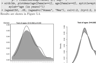
5.4 Density plot of age by gender . . . 111
6.1 Scatterplot of observed values for age and I1 (plus smoothers by substance) 130 6.2 SAS table produced withlatexdestination inODS . . . 134
6.3 Q-Q plot from SAS, default diagnostics from R . . . 137
6.4 Empirical density of residuals, with superimposed normal density . . . 137
6.5 Interaction plot of CESD as a function of substance group and gender . . . 140
6.6 Boxplot of CESD as a function of substance group and gender . . . 140
6.7 Pairwise comparisons . . . 146
7.1 Scatterplots of smoothed association of PCS with CESD . . . 186
7.2 Side-by-side box plots of CESD by treatment and time . . . 193
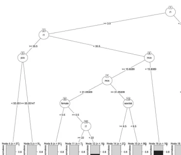
7.3 Recursive partitioning tree from R . . . 206
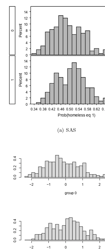
7.4 Graphical display of assignment probabilities or score functions from linear discriminant analysis by actual homeless status . . . 209
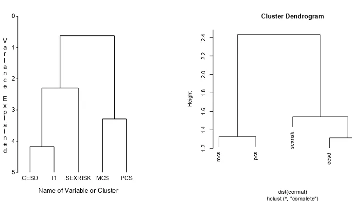
7.5 Results from hierarchical clustering . . . 210
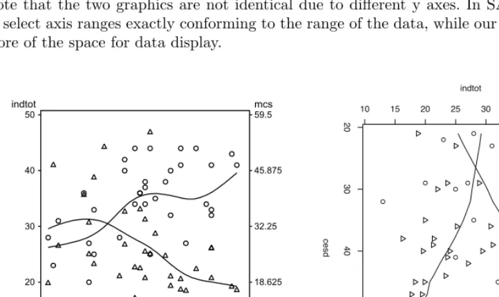
8.1 Plot of InDUC and MCS vs. CESD for female alcohol-involved subjects . . 231
8.2 Association of MCS and CESD, stratified by substance and report of suicidal thoughts . . . 233
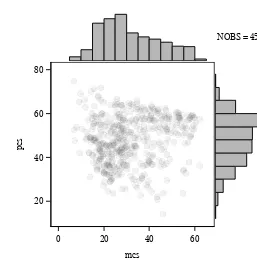
8.3 Association of MCS and CESD with marginal histograms . . . 234
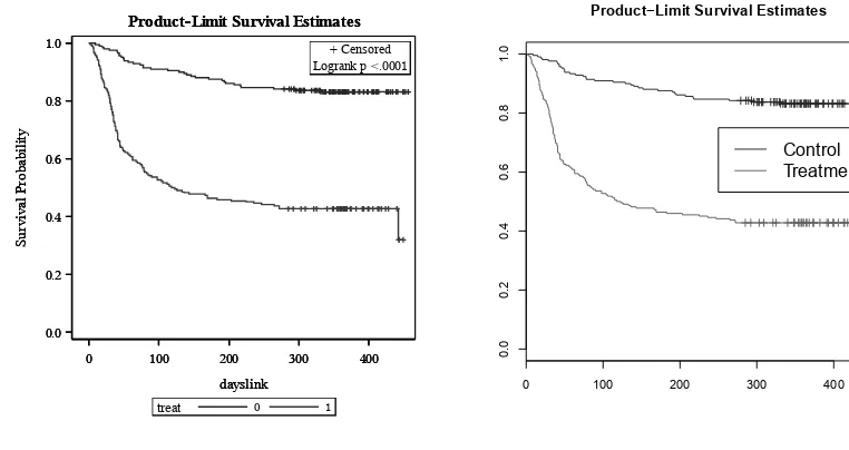
8.4 Kaplan–Meier estimate of time to linkage to primary care by randomization group . . . 236
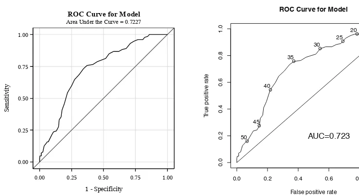
8.5 Receiver operating characteristic curve for the logistical regression model pre-dicting suicidal thoughts using the CESD as a measure of depressive symp-toms (sensitivity = true positive rate; 1-specificity = false positive rate) . . 237
8.6 Pairsplot of variables from the HELP dataset . . . 238
8.7 Visual display of correlations and associations . . . 240
10.1 Plot of true and simulated distributions . . . 274
xviii LIST OF FIGURES
11.1 Sample Markdown input file . . . 288
11.2 Formatted output from R Markdown example . . . 289
12.1 Running average for Cauchy andt distributions . . . 320
12.2 Massachusetts counties . . . 324
12.3 Bike plot with map background . . . 326
12.4 Choropleth map . . . 329
12.5 Sales plot . . . 334
12.6 Number of flights departing Bradley airport on Mondays over time . . . 338
A.1 SAS Windows interface . . . 342
A.2 Running a SAS program . . . 343
A.3 Results fromproc print . . . 344
A.4 Results fromproc univariate . . . 345
A.5 The SAS window after running the sample session code . . . 346
A.6 The SAS Explorer window . . . 347
A.7 Opening the on-line help . . . 348
A.8 The SAS Help and Documentation window . . . 348
B.1 R Windows graphical user interface . . . 358
B.2 R Mac OS X graphical user interface . . . 359
B.3 RStudio graphical user interface . . . 360
B.4 Sample session in R . . . 361
B.5 Documentation on themean()function . . . 363
List of Tables
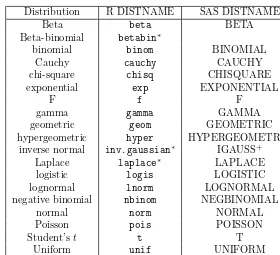
3.1 Quantiles, probabilities, and pseudo-random number generation:
distribu-tions available in SAS and R . . . 54
6.1 Formatted results using thextablepackage . . . 134
7.1 Generalized linear model distributions supported by SAS and R . . . 150
11.1 Bayesian modeling functions available within theMCMCpackpackage . . . . 292
12.1 Weights, volume, and values for the knapsack problem . . . 337
B.1 CRAN task views . . . 373
C.1 Analyses undertaken using the HELP dataset . . . 379
C.2 Annotated description of variables in the HELP dataset . . . 381
Preface to the second edition
Software systems evolve, and so do the approaches and expertise of statistical analysts. After the publication of the first edition of SAS and R: Data Management, Statistical
Analysis, and Graphics, we began a blog in which we explored many new case studies and
applications, ranging from generating a Fibonacci series to fitting finite mixture models with concomitant variables. We also discussed some additions to SAS and new or improved R packages. The blog now has hundreds of entries and (according to Google Analytics) has received hundreds of thousands of visits.
The volume you are holding is nearly 50% longer than the first edition, and much of the new material is adapted from these blog entries, while it also includes other improvements and additions which have emerged in the last few years.
We have extensively reorganized the material in the book and created three new chapters. The first,Simulation, includes examples where data are generated from complex models such as mixed effects models and survival models, and from distributions using the Metropolis– Hastings algorithm. We also explore three interesting statistics and probability examples via simulation. The second isSpecial topics, where we describe some key features, such as processing by group, and detail several important areas of statistics, including Bayesian methods, propensity scores, and bootstrapping. The last isCase studies, where we demon-strate examples of some data management tasks, read complex files, make and annotate maps, and show how to “scrape” data from web pages.
We also cover some important new tools, including the use of RStudio, a powerful and easy-to-use front end for R that adds innumerable features to R. In our experience, it at least doubles the productivity of R users, and our SAS-using students find it an extremely comfortable interface that bears some similarity to the SAS GUI.
We have added a separate section and examples that describe “reproducible analysis.” This is the notion that code, results, and interpretation should live together in a single place. We used two reproducible analysis systems (SASweave and Sweave) to generate the example code and output in the book. Code extracted from these files is provided on the book web site. In this edition, we provide a detailed discussion of the philosophy and use of these systems. In particular, we feel that theknitrandmarkdownpackages for R, which are tightly integrated with RStudio, should become a part of every R user’s toolbox. We can’t imagine working on a project without them.
Finally, we’ve reorganized much of the material from the first edition into smaller, more focused chapters. Users will now find separate (and enhanced) chapters on data input and output, data management, statistical and mathematical functions, and programming, rather than a single chapter on “data management.” Graphics are now discussed in two chapters: one on high-level types of plots, such as scatterplots and histograms, and another on cus-tomizing the fine details of the plots, such as the number of tick marks and the color of plot symbols.
We’re immensely gratified by the positive response the first edition elicited, and hope the current volume will be as useful to you.
xxii PREFACE
On the web
The book website athttp://www.amherst.edu/~nhorton/sasr2includes the table of con-tents, the indices, the HELP dataset, example code in SAS and R, a pointer to the blog, and a list of errata.
Acknowledgments
In addition to those acknowledged in the first edition, we would like to thank Kathryn Aloisio, Gregory Call, J.J. Allaire and the RStudio developers, plus the many individuals who have created and shared R packages or SAS macros. Their contributions to SAS, R, or LATEX programming efforts, comments, guidance, and/or helpful suggestions on drafts of
the revision have been extremely helpful. Above all we greatly appreciate Sara and Julia as well as Abby, Alana, Kinari, and Sam, for their patience and support.
Preface to the first edition
SASTM (SAS Institute [153]) and R (R development core team [135]) are two statistical
software packages used in many fields of research. SAS is commercial software developed by SAS Institute; it includes well-validated statistical algorithms. It can be licensed but not purchased. Paying for a license entitles the licensee to professional customer support. However, licensing is expensive and SAS sometimes incorporates new statistical methods only after a significant lag. In contrast, R is free, open-source software, developed by a large group of people, many of whom are volunteers. It has a large and growing user and developer base. Methodologists often release applications for general use in R shortly after they have been introduced into the literature. Professional customer support is not provided, though there are many resources for users. There are settings in which one of these useful tools is needed, and users who have spent many hours gaining expertise in the other often find it frustrating to make the transition.
We have written this book as a reference text for users of SAS and R. Our primary goal is to provide users with an easy way to learn how to perform an analytic task in both systems, without having to navigate through the extensive, idiosyncratic, and sometimes (often?) unwieldy documentation each provides. We expect the book to function in the same way that an English–French dictionary informs users of both the equivalent nouns and verbs in the two languages as well as the differences in grammar. We include many common tasks, including data management, descriptive summaries, inferential procedures, regression analysis, multivariate methods, and the creation of graphics. We also show some more complex applications. In toto, we hope that the text will allow easier mobility between systems for users of any statistical system.
We do not attempt to exhaustively detail all possible ways available to accomplish a given task in each system. Neither do we claim to provide the most elegant solution. We have tried to provide a simple approach that is easy to understand for a new user, and have supplied several solutions when they seem likely to be helpful. Carrying forward the analogy to an English–French dictionary, we suggest language that will communicate the point effectively, without listing every synonym or providing guidance on native idiom or eloquence.
Who should use this book
Those with an understanding of statistics at the level of multiple-regression analysis will find this book helpful. This group includes professional analysts who use statistical packages almost every day as well as statisticians, epidemiologists, economists, engineers, physicians, sociologists, and others engaged in research or data analysis. We anticipate that this tool will be particularly useful for sophisticated users, those with years of experience in only one system, who need or want to use the other system. However, intermediate-level analysts should reap the same benefit. In addition, the book will bolster the analytic abilities of a relatively new user of either system, by providing a concise reference manual and annotated examples executed in both packages.
xxiv PREFACE
Using the book
The book has three indices, in addition to the comprehensive Table of Contents. These include: 1) a detailed topic (subject) index in English; 2) a SAS index, organized by SAS syntax; and 3) an R index, describing R syntax. SAS users can use the SAS index to look up a task for which they know the SAS code and turn to a page with that code as well as the associated R code to carry out that task. R users can use the dictionary in an analogous fashion using the R index.
Extensive example analyses are presented; see Table C.1 for a comprehensive list. These employ a single dataset (from the HELP study), described in Appendix C. Readers are encouraged to download the dataset and code from the book website. The examples demon-strate the code in action and facilitate exploration by the reader.
Differences between SAS and R
SAS and R are so fundamentally distinct that an enumeration of their differences would be counterproductive. However, some differences are important for new users to bear in mind.
SAS includes data management tools that are primarily intended to prepare data for analysis. After preparation, analysis is performed in a distinct step, the implementation of which effectively cannot be changed by the user, though often extensive options are available. R is a programming environment tailored for data analysis. Data management and analysis are integrated. This means, for example, that calculating body mass index (BMI) from weight and height can be treated as a function of the data, and as such is as likely to appear within a data analysis as in making a “new” piece of data to keep.
SAS Institute makes decisions about how to change the software or expand the scope of included analyses. These decisions are based on the needs of the user community and on corporate goals for profitability. For example, when changes are made, backwards com-patibility is almost always maintained, and documentation of exceptions is extensive. SAS Institute’s corporate conservatism means that techniques are sometimes not included in SAS until they have been discussed in the peer-reviewed literature for many years. While the R core team controls base functionality, a very large number of users have developed functions for R. Methodologists often release R functions to implement their work concurrently with publication. While this provides great flexibility, it comes at some cost. A user-contributed function may implement a desired methodology, but code quality may be unknown, docu-mentation scarce, and paid support nonexistent. Sometimes a function which once worked may become defunct due to a lack of backwards compatibility and/or the author’s inability to, or lack of interest in, updating it.
Other differences between SAS and R are worth noting. Data management in SAS is undertaken using row by row (observation-level) operations. R is inherently a vector-based language, where columns (variables) are manipulated. R is case sensitive, while SAS is generally not.
Where to begin
PREFACE xxv
On the web
The book website includes the Table of Contents, the indices, the HELP dataset, example code in SAS and R, and a list of errata.
Acknowledgments
We would like to thank Rob Calver, Shashi Kumar, and Sarah Morris for their support and guidance at Informa CRC/Chapman and Hall, the Department of Statistics at the University of Auckland for graciously hosting NH during a sabbatical leave, and the Office of the Provost at Smith College. We also thank Allyson Abrams, Tanya Hakim, Ross Ihaka, Albyn Jones, Russell Lenth, Brian McArdle, Paul Murrell, Alastair Scott, David Schoenfeld, Duncan Temple Lang, Kristin Tyler, Chris Wild, and Alan Zaslavsky for contributions to SAS, R, or LATEX programming efforts, comments, guidance, and/or helpful suggestions on
drafts of the manuscript.
Above all we greatly appreciate Sara and Julia as well as Abby, Alana, Kinari, and Sam, for their patience and support.
Chapter 1
Data input and output
This chapter reviews data input and output, including reading and writing files in spread-sheet, ASCII file, native, and foreign formats.
1.1
Input
Both SAS and R provide comprehensive support for data input and output. In this section we address aspects of these tasks.
SAS native datasets are rectangular files with data stored in a special format. They have the formfilename.sas7bdator something similar, depending on version. In the fol-lowing, we assume that files are stored in directories and that the locations of the direc-tories in the operating system can be labeled using Windows syntax (though SAS allows UNIX/Linux/Mac OS X-style forward slash as a directory delimiter on Windows). Other operating systems will use local idioms in describing locations.
R organizes data in dataframes (B.4.6), or connected series of rectangular arrays, which can be saved as platform independent objects. R also allows UNIX-style directory delimiters (forward slash) on Windows.
1.1.1
Native dataset
Example:7.10
SAS
libname libref "dir_location"; data ds;
set libref.sasfilename; /* Note: no file extension */ ...
run;
or
data ds;
set "dir_location\sasfilename.sas7bdat"; /* Windows only */ set "dir_location/sasfilename.sas7bdat";
/* works on all OS including Windows */ ...
run;
Note: The filesasfilename.sas7bdat is created by using alibref in a data statement;
see 1.2.3.
2 CHAPTER 1. DATA INPUT AND OUTPUT
R
load(file="dir_location/savedfile") # works on all OS including Windows load(file="dir_location\\savedfile") # Windows only
Note:Forward slash is supported as a directory delimiter on all operating systems; a double
backslash is supported under Windows. The filesavedfileis created bysave()(see 1.2.3). Running the command print(load(file="dir location/savedfile")) will display the objects that are added to the workspace.
1.1.2
Fixed format text files
See 1.1.4 (read more complex fixed files) and 12.2 (read variable format files).
SAS
data ds;
infile 'C:\file_location\filename.ext'; input varname1 ... varnamek;
run;
or
filename filehandle 'file_location/filename.ext';
proc import datafile=filehandle out=ds dbms=dlm;
getnames=yes; run;
Note: The infile approach allows the user to limit the number of rows read from the
data file using theobsoption. Character variables are noted with a trailing ‘$’, e.g., use a statement such asinput varname1 varname2 $ varname3if the second position contains a character variable (see 1.1.4 for examples). Theinputstatement allows many options and can be used to read files with variable format (12.2).
In proc import, thegetnames=yes statement is used if the first row of the input file contains variable names (the variable types are detected from the data). If the first row does not contain variable names then the getnames=no option should be specified. The
guessingrowsoption (not shown) will base the variable formats on other than the default 20 rows. Theproc import statement will accept an explicit file location rather than a file associated by thefilenamestatement as in 7.10.
Note that in Windows installations, SAS accepts either slashes or backslashes to de-note directory structures. For Linux, only forward slashes are allowed. Behavior in other operating systems may vary.
In addition to these methods, files can be read by selecting theImport Dataoption on thefile menu in the GUI.
R
ds = read.table("dir_location\\file.txt", header=TRUE) # Windows only
or
ds = read.table("dir_location/file.txt", header=TRUE) # all OS (including # Windows)
Note: Forward slash is supported as a directory delimiter on all operating systems; a double
backslash is supported under Windows. If the first row of the file includes the name of the variables, these entries will be used to create appropriate names (reserved characters such as
1.1. INPUT 3 through thenrowsoption. Theread.table()function can support reading from a URL as a filename (see 1.1.12) or browse files interactively usingfile.choose()(see 4.3.7).
1.1.3
Other fixed files
See 1.1.4 (read more complex fixed files) and 12.2 (read variable format files).
Sometimes data arrives in files that are very irregular in shape. For example, there may be a variable number of fields per line, or some data in the line may describe the remainder of the line. In such cases, a useful generic approach is to read each line into a single character variable, then use character variable functions (see 2.2) to extract the contents.
SAS
data ds;
data filenames;
infile "file_location/file.txt"; input var1 $32767.;
run;
Note: The$32767.allows input lines as long as 32,767 characters, the maximum length of
SAS character variables.
R
ds = readLines("file.txt")
or
ds = scan("file.txt")
Note:ThereadLines()function returns a character vector with length equal to the number
of lines read (seefile()). A limit on the number of lines to be read can be specified through thenrows option. The scan() function returns a vector, with entries separated by white space by default. These functions read by default from standard input (see stdin()and
?connections), but can also read from a file or URL (see 1.1.12). Theread.fwf()function may also be useful for reading fixed width files. The capture.output() function can be used to send output to a character string or file (see alsosink()).
1.1.4
Reading more complex text files
See 1.1.2 (read fixed files) and 12.2 (read variable format files).
Text data files often contain data in special formats. One common example is date variables. Special values can be read in using informats (A.6.3). As an example below we consider the following data.
1 AGKE 08/03/1999 $10.49 2 SBKE 12/18/2002 $11.00 3 SEKK 10/23/1995 $5.00
SAS
data ds;
infile 'C:\file_location\filename.dat';
input id initials $ datevar mmddyy10. cost dollar7.4; run;
Note: The SAS informats (A.6.3) denoted by the mmddyy10. and dollar7.4 inform the
4 CHAPTER 1. DATA INPUT AND OUTPUT
treated as numbers or letters, but read and interpreted according to the rules specified. In the case ofdatevar, SAS reads the date appropriately and stores a SAS date value (A.6.3). For cost, SAS ignores the ‘$’ in the data and would also ignore commas, if they were present. Theinput statement allows many options for additional data formats and can be used to read files with variable format (12.2).
Other common features of text data files include very long lines and missing data. These are addressed through theinfile or filenamestatements. Missing data may require the
missoveroption to the infilestatement as well as listing the columns in which variables appear in the dataset in theinputstatement. Long lines (many columns in the data file) may require thelrecl option to the infile or filenamestatement. For a thorough dis-cussion, see the on-line help: Contents; SAS Products; Base SAS; SAS Language Reference: Concepts; DATA Step Concepts; Reading Raw Data; Reading Raw Data with the INPUT statement.
R
tmpds = read.table("file_location/filename.dat") id = tmpds$V1
initials = tmpds$V2
datevar = as.Date(as.character(tmpds$V3), "%m/%d/%Y") cost = as.numeric(substr(tmpds$V4, 2, 100))
ds = data.frame(id, initials, datevar, cost) rm(tmpds, id, initials, datevar, cost)
Note: In R, this task is accomplished by first reading the dataset (with default names
from read.table() denoted V1 through V4). These objects can be manipulated using
as.character()to undo the default coding as factor variables, and coerced to the appro-priate data types. For the costvariable, the dollar signs are removed using the substr()
function. Finally, the individual variables are gathered together as a dataframe.
1.1.5
Comma separated value (CSV) files
Example:2.6.1
SAS
data ds;
infile 'dir_location\filename.csv' delimiter=','; input varname1 ... varnamek;
run;
or
proc import datafile='dir_location\full_filename' out=ds dbms=csv;
delimiter=','; getnames=yes; run;
Note: Character variables are noted with a trailing ‘$’, e.g., use a statement such as
input varname1 varname2 $ varname3 if the second column contains characters. The
proc import syntax allows for the first row of the input file to contain variable names, with variable types detected from the data. If the first row does not contain variable names then usegetnames=no.
1.1. INPUT 5
R
ds = read.csv("dir_location/file.csv")
Note: The stringsAsFactorsoption can be set to prevent automatic creation of factors
for categorical variables. A limit on the number of lines to be read can be specified through the nrows option. The command read.csv(file.choose()) can be used to browse files interactively (see 4.3.7). The comma-separated file can be given as a URL (see 1.1.12). The
colClassesoption can be used to speed up reading large files.
1.1.6
Read sheets from an Excel file
SAS
proc import out=ds
datafile="dir_location\full_filename" dbms=excel replace; range="sheetname$a1:zz4000";
getnames=yes; mixed=no; usedate=yes; scantext=yes; run;
Note: Therangeoption specifies the sheet name and cells to select within the Excel
work-book. The $ after the sheet name indicates that a range of cells follows; without it the entire sheet is read. Thea1:zz4000gives the upper left and lower right cells of the region to be read, separated by a colon. The getnames option indicates whether the names are included in the first row. Ifmixed=yes(default isno) then numeric values are converted to character if any values are character. Ifusedate=yesthen Excel date values are converted to SAS date values. If scantext=yes then SAS checks for the longest character value in the Excel data and sets the SAS character value length accordingly. Note that the dbms
option also accepts the values excelcs and xls, either of which may be helpful in some settings. Documentation is found in SAS Products; SAS/ACCESS; SAS/ACCESS Interface to PC files: Reference; Import and Export Wizards and Procedures; File Format-Specific Reference for the IMPORT and EXPORT Procedures.
R
library(gdata)
ds = read.xls("http://www.amherst.edu/~nhorton/sasr2/datasets/help.xlsx", sheet=1)
Note: In this implementation, the sheet number is provided, rather than name.
1.1.7
Read data from R into SAS
The R packageforeignincludes thewrite.dbf()function; we recommend this as a reliable format for extracting data from R into a SAS-ready file, though other options are possible. Then SAS proc import can easily read the DBF file. Because we describe moving from R to SAS, we begin with the R entry.
R
tosas = data.frame(ds) library(foreign)
write.dbf(tosas,"dir_location/tosas.dbf")
SAS
proc import datafile="dir_location\tosas.dbf" out=fromr dbms=dbf;
6 CHAPTER 1. DATA INPUT AND OUTPUT
1.1.8
Read data from SAS into R
SAS
proc export data=ds
outfile = "dir_location\to_r.dbf" dbms=dbf; run;
R
library(foreign)
ds = read.dbf("dir_location/to_r.dbf")
or
library(sas7bdat)
helpfromSAS = read.sas7bdat("dir_location/help.sas7bdat")
Note: The first set of code (obviously) requires a working version of SAS. The second can
be used with any SAS formatted data set; it is based on reverse-engineering of the SAS data set format, which SAS has not made public.
1.1.9
Reading datasets in other formats
Example:6.6.1
SAS
libname ref spss 'filename.sav'; /* SPSS */ libname ref bmdp 'filename.dat'; /* BMDP */
libname ref v6 'filename.ssd01; /* SAS vers. 6 */ libname ref xport 'filename.xpt'; /* SAS export */ libname ref xml 'filename.xml'; /* XML */
data ds;
set ref.filename; run;
or
proc import datafile="filename.ext' out=ds
dbms=excel; /* Excel */
run;
... dbms=access; ... /* Access */
... dbms=dta; ... /* Stata */
Note: Thelibnamestatements above refer to files, rather than directories. The extensions
shown above are those typically used for these file types, but in any event the full name of the file, including the extension, is needed in thelibnamestatement. In contrast, only the file name (without the extension) is used in thesetstatement. The data type options specified above in thelibnamestatement anddbms option are available in most operating systems. To see what data types are available, check the on-line help. For Windows: Contents, Using SAS Software in Your Operating Environment, SAS Companion for Windows, Features of the SAS language for Windows, SAS Statements under Windows, LIBNAME statement.
1.1. INPUT 7
R
library(foreign)
ds = read.dbf("filename.dbf") # DBase ds = read.epiinfo("filename.epiinfo") # Epi Info
ds = read.mtp("filename.mtp") # Minitab portable worksheet ds = read.octave("filename.octave") # Octave
ds = read.ssd("filename.ssd") # SAS version 6 ds = read.xport("filename.xport") # SAS XPORT file ds = read.spss("filename.sav") # SPSS
ds = read.dta("filename.dta") # Stata ds = read.systat("filename.sys") # Systat
Note: Theforeignpackage can read Stata, Epi Info, Minitab, Octave, SPSS, and Systat
files (with the caveat that SAS files may be platform dependent). Theread.ssd()function will only work if SAS is installed on the local machine.
1.1.10
Reading data with a variable number of words in a field
Reading data in a complex data format will generally require a tailored approach. Here we give a relatively simple example and outline the key tools useful for reading in data in complex formats. Suppose we have data as follows:
1 Las Vegas, NV --- 53.3 --- --- 1 2 Sacramento, CA --- 42.3 --- --- 2 3 Miami, FL --- 41.8 --- --- 3 4 Tucson, AZ --- 41.7 --- --- 4 5 Cleveland, OH --- 38.3 --- --- 5 6 Cincinnati, OH 15 36.4 --- --- 6
7 Colorado Springs, CO --- 36.1 --- --- 7 8 Memphis, TN --- 35.3 --- --- 8
8 New Orleans, LA --- 35.3 --- --- 8 10 Mesa, AZ --- 34.7 --- --- 10 11 Baltimore, MD --- 33.2 --- --- 11 12 Philadelphia, PA --- 31.7 --- --- 12 13 Salt Lake City, UT --- 31.9 17 --- 13
The --- means that the value is missing. Note two complexities here. First, fields are delimited by both spaces and commas, where the latter separates the city from the state. Second, cities may have names consisting of more than one word.
SAS
data ds;
infile "dir_location/cities.txt" dlm=", "; input id city & $20. state $2. v1 - v5; run;
Note: Theinfileandinputstatements in the data step can accommodate many features
of text files. Thedlm=", "tells SAS that both commas and spaces are delimiters in this file. In theinputstatement, the instructioncity @ $20.is parsed as: read up to 20 characters, and within that distance, spaces should not be considered delimiters. In this example, the
---are interpreted by SAS as “invalid data” but are recorded in thedsdata set as missing values.
8 CHAPTER 1. DATA INPUT AND OUTPUT
R
readcities = function(thisline) { thislen = length(thisline) id = as.numeric(thisline[1])
v1 = as.numeric(thisline[thislen-4]) v2 = as.numeric(thisline[thislen-3]) v3 = as.numeric(thisline[thislen-2]) v4 = as.numeric(thisline[thislen-1]) v5 = as.numeric(thisline[thislen])
city = paste(thisline[2:(thislen-5)], collapse=" ")
return(list(id=id,city=city,v1=v1,v2=v2,v3=v3,v4=v4,v5=v5)) }
file
= readLines("http://www.amherst.edu/~nhorton/sasr2/datasets/cities.txt") split = strsplit(file, " ") # split up fields for each line
as.data.frame(t(sapply(split, readcities)))
Note:In R, we first write a function that processes a line and converts each field other than
the city name into a numeric variable. The function works backwards from the end of the line to find the appropriate elements, then calculates what is left over to store in the city variable. We need each line to be converted into a character vector containing each “word” (character strings divided by spaces) as a separate element. We’ll do this by first reading each line, then splitting it into words. This results in a list object, where the items in the list are the vectors of words. Then we can call thereadcities()function for each vector using an invocation ofsapply()(B.5.2), which avoids use of aforloop. The resulting object is transposed then coerced into a dataframe (see alsocount.fields()).
1.1.11
Read a file byte by byte
It may be necessary to read data that is not stored in ASCII (or other text) format. At such times, it may be useful to read the raw bytes stored in the file.
SAS
data test;
infile "dir_location/full_filename" recfm=n; input byte ib1. @@;
run
Note: Therecfm=noption tells SAS to read the file in binary; note that this may differ by
OS. Theib1. informat tells SAS to read one byte. The @@tells SAS to hold this line of input, rather than skipping to a new line, when data is read. A new line will be begun only when the current line is finished. SAS will read bytes until there are no more to read. Other tools can then be used to assemble the bytes into usable data.
R
finfo = file.info("full_filename") toread = file("full_filename", "rb")
alldata = readBin(toread, integer(), size=1, n=finfo$size, endian="little")
Note:In R, thereadBin()function is used to read the file, after some initial prep work. The
1.1. INPUT 9 of the elements, in bytes, and the endian option helps describe how the bytes should be read.
1.1.12
Access data from a URL
Examples:5.7.1 and 12.4.2
SAS
filename myurl url "https://example.com/file.txt";
proc import datafile=myurl out=ds dbms=filetype; run;
Note:If the URL requires a username and password, thefilenamestatement acceptsuser=
andpass=options. The url “handle”, heremyurl, can be no longer than 8 characters. The url handle can be used in animportprocedure as shown, or with aninfilestatement in a
datastep (see 12.2). Theimport procedure supports manyfiletypes, as shown in 1.1.2, 1.1.5, 1.1.6, 1.1.7, and 1.1.9.
R
library(RCurl)
myurl = getURL("https://example.com/file.txt") ds = readLines(textConnection(myurl))
Note: ThereadLines()function reads arbitrary text, whileread.table()can be used to
read a file with cases corresponding to lines and variables to fields in the file (theheader
option sets variable names to entries in the first line). To read Hypertext Transfer Pro-tocol Secure (https) URLs, the getURL() function from the RCurl package is needed in conjunction with thetextConnection() function (see alsourl()). Access through proxy servers as well as specification of username and passwords is provided by the function
download.file(). A limit on the number of lines to be read can be specified through the
nrowsoption.
1.1.13
Read an XML-formatted file
A sample (flat) XML form of the HELP dataset can be found at http://www.amherst. edu/~nhorton/sasr2/datasets/help.xml. The first ten lines of the file consist of:
<?xml version="1.0" encoding="iso-8859-1" ?> <TABLE>
<HELP>
<id> 1 </id>
<e2b1 Missing="." /> <g1b1> 0 </g1b1> <i11 Missing="." /> <pcs1> 54.2258263 </pcs1> <mcs1> 52.2347984 </mcs1> <cesd1> 7 </cesd1>
10 CHAPTER 1. DATA INPUT AND OUTPUT
SAS
libname ref xml 'dir_location\filename.xml';
data ds;
set ref.filename_without_extension; run;
Note: The libnamestatement above refers to a file name, rather than a directory name.
The “xml” extension is typically used for this file type, but in any event the full name of the file, including the extension, is needed.
R
library(XML)
urlstring = "http://www.amherst.edu/~nhorton/sasr2/datasets/help.xml" doc = xmlRoot(xmlTreeParse(urlstring))
tmp = xmlSApply(doc, function(x) xmlSApply(x, xmlValue)) ds = t(tmp)[,-1]
Note: The XMLpackage provides support for reading XML files. The xmlRoot() function
opens a connection to the file, whilexmlSApply()andxmlValue()are called recursively to process the file. The returned object is a character matrix with columns corresponding to observations and rows corresponding to variables, which in this example are then transposed (see alsoreadHTMLTable()).
1.1.14
Manual data entry
SAS
data ds; input x1 x2; cards; 1 2 1 3 1.4 2 123 4.5 ; run;
Note:The above code demonstrates reading data into a SAS dataset within a SAS program.
The semicolon following the data terminates thedata step, meaning that arunstatement is not actually required. The inputstatement used above employs the syntax discussed in 1.1.2. In addition to this option for entering data within SAS, there is a GUI-based data entry/editing tool called the Table Editor. It can be accessed using the mouse through the Tools menu, or by using the viewtablecommand on the SAS command line.
R
x = numeric(10) data.entry(x)
or
x1 = c(1, 1, 1.4, 123) x2 = c(2, 3, 2, 4.5)
Note: Thedata.entry()function invokes a spreadsheet that can be used to edit or
1.2. OUTPUT 11 which leaves the objects given as argument unchanged, returning a new object with the desired edits (see also thefix()function).
1.2
Output
1.2.1
Displaying data
Example:6.6.2
See 2.1.3 (values of variables in a dataset).
SAS
title1 'Display of variables'; footnote1 'A footnote';
proc print data=ds; var x1 x3 xk x2; format x3 dollar10.2; run;
Note:Forproc printthevarstatement selects variables to be included. The format
state-ment, as demonstrated, can alter the appearance of the data; herex3is displayed as a dollar
amount with 10 total digits, two of them to the right of the decimal. The keyword numeric
can replace the variable name and will cause all of the numerical variables to be displayed in the same format. See A.6.3 for further discussion, as well as A.6.2, 11.1, and A.6.1 for ways to limit which observations are displayed. The var statement, as demonstrated, ensures the variables are displayed in the desired order. Thetitle andfootnote statements and related statementstitle1,footnote2, etc., allow headers and footers to be added to each output page. Specifying the command with no argument will remove the title or footnote from subsequent output.
SAS also providesproc reportandproc tabulateto create more customized output.
R
dollarcents = function(x)
return(paste("$", format(round(x*100, 0)/100, nsmall=2), sep="")) data.frame(x1, dollarcents(x3), xk, x2)
or
ds[,c("x1", "x3", "xk", "x2")]
Note: A function can be defined to format a vector as U.S. dollar and cents by using the
round()function (see 3.2.4) to control the number of digits (2) to the right of the decimal. Alternatively, named variables from a dataframe can be printed. Thecat()function can be used to concatenate values and display them on the console (or route them to a file using the
fileoption). More control on the appearance of printed values is available through use of
format()(control of digits and justification),sprintf()(use of C-style string formatting) andprettyNum()(another routine to format using C-style specifications).
1.2.2
Number of digits to display
Example:2.6.1
12 CHAPTER 1. DATA INPUT AND OUTPUT
R
options(digits=n)
Note: The options(digits=n) command can be used to change the default number of
decimal places to display in subsequent R output. To affect the actual significant digits in the data, use theround()function (see 3.2.4).
1.2.3
Save a native dataset
Example:2.6.1
SAS
libname libref "dir_location";
data libref.sasfilename; set ds;
run;
Note: A SAS dataset can be read back into SAS using asetstatement with alibref(see
1.1.1).
R
save(robject, file="savedfile")
Note: An object (typically a dataframe or a list of objects) can be read back into R using
load()(see 1.1.1).
1.2.4
Creating datasets in text format
SAS
proc export data=ds outfile='file_location_and_name'
dbms=csv; /* comma-separated values */
...dbms=tab; /* tab-separated values */
...dbms=dlm; /* arbitrary delimiter; default is space,
others with delimiter= statement */
R
write.csv(ds, file="full_file_location_and_name")
or
library(foreign)
write.table(ds, file="full_file_location_and_name")
Note:Thesepoption towrite.table()can be used to change the default delimiter (space)
to an arbitrary value.
1.2.5
Creating Excel spreadsheets
SAS
data help;
set "c:\book\help.sas7bdat"; run;
proc export data=ds outfile="dir_location/filename.xls" dbms=excel;
1.2. OUTPUT 13 or
proc export data=ds
outfile = "dir_location/filename.xls" dbms=excel; sheet="sheetname";
run;
Note: The latter code demonstrates adding a sheet to an existing Excel workbook.
Docu-mentation can be found at SAS Products; SAS/ACCESS; SAS/ACCESS Interface to PC files: Reference; Import and Export Wizards and Procedures; File Format-Specific Reference for the IMPORT and EXPORT Procedures.
There are several other methods for doing this in SAS. A possibly simpler way would be to use thelibnamestatement, but platform dependence makes this method less desirable.
R
library(WriteXLS)
HELP = read.csv("http://www.amherst.edu/~nhorton/sasr2/datasets/help.csv") WriteXLS("HELP", ExcelFileName="newhelp.xls")
Note: TheWriteXLSpackage provides this functionality. It uses Perl (Practical extraction
and report language,http://www.perl.org) and requires an external installation of Perl to function. After installing Perl, this requires running the operating system commandcpan -i Text::CSV XSat the command line.
1.2.6
Creating files for use by other packages
Example:2.6.1
See also 1.2.8 (write XML).
SAS
libname ref spss 'filename.sav'; /* SPSS */ libname ref bmdp 'filename.dat'; /* BMDP */
libname ref v6 'filename.ssd01'; /* SAS version 6 */ libname ref xport 'filename.xpt'; /* SAS export */ libname ref xml 'filename.xml'; /* XML */
data ref.filename_without_extension; set ds;
or
proc export data=ds outfile='file_location_and_name'
dbms=csv; /* comma-separated values */
...dbms=dbf; /* dbase 5,IV,III */
...dbms=excel; /* excel */
...dbms=dta; /* Stata */
...dbms=tab; /* tab-separated values */
...dmbs=access; /* Access table */
...dbms=dlm; /* arbitrary delimiter; default is space,
others with delimiter=char statement */
Note: The libname statements above refer to file names, rather than directory names.
14 CHAPTER 1. DATA INPUT AND OUTPUT
R
library(foreign)
write.dta(ds, "filename.dta") write.dbf(ds, "filename.dbf")
write.foreign(ds, "filename.dat", "filename.sas", package="SAS")
Note:Support for writing dataframes in R is provided in theforeignpackage. It is possible
to write files directly in Stata format (seewrite.dta()) or DBF format (seewrite.dbf()) or create files with fixed fields as well as the code to read the file from within Stata, SAS, or SPSS using write.foreign().
As an example with a dataset with two numeric variables X1 and X2, the call to
write.foreign()creates one file with the data and the SAS command filefilename.sas, with the following contents.
data ds;
infile "file.dat" dsd lrecl=79; input x1 x2;
run;
This code uses proc format (2.2.19) statements in SAS to store string (character) variables. Similar code is created for SPSS using write.foreign() with the appropriate
packageoption.
1.2.7
Creating HTML formatted output
SAS
ods html file="filename.html"; ...
ods html close;
Note:Any output generated between anods htmlstatement and anods html close
state-ment will be included in an HTML (hyper-text markup language) file (A.7.2). By default this will be displayed in an internal SAS window; the optional file option shown above will cause the output to be saved as a file.
R
library(prettyR)
htmlize("script.R", title="mytitle", echo=TRUE)
Note: Thehtmlize()function within theprettyRpackage can be used to produce HTML
(hypertext markup language) from a script file (see B.2.1). Thecat()function is used inside the script file (here denoted by script.R) to generate output. The hwriterpackage also supports writing R objects in HTML format. In addition, the R Markdown system using theknitr package and the knit2html()function can create HTML files as an option for reproducible analysis (11.3).
1.2.8
Creating XML datasets and output
SAS
libname ref xml 'dir_location\filename.xml';
data ref.filename_without_extension; set ds;
1.3. FURTHER RESOURCES 15 or
ods docbook file='filename.xml'; ...
ods close;
Note:Thelibnamestatement can be used to write a SAS dataset to an XML-formatted file.
It refers to a file name, rather than a directory name. The file extensionxmlis conventionally used but thexmlspecification, rather than the file extension, determines the file type that is created.
Theods docbookstatement, in contrast, can be used to generate an XML file displaying procedure output; the file is formatted according to the OASIS DocBook DTD (document type definition).
R
In R, theXMLpackage provides support for writing XML files (see 1.1.9, write foreign files and Further resources).
1.3
Further resources
Introductions to data input and output in SAS can be found in [32] and [25]. Similar developments in R are accessibly presented in [187]. Paul Murrell’s Introduction to Data
Technologies text [124] provides a comprehensive introduction to XML, SQL, and other