Reflectors
Xi Xiong, Justin Chan
1, Ethan Yu, Nisha Kumari, Ardalan Amiri Sani
2, Changxi Zheng
3, Xia Zhou
Dartmouth College,1University of Washington,2UC Irvine,3Columbia University
ABSTRACT
Judicious control of indoor wireless coverage is crucial in built environments. It enhances signal reception, reduces harmful in-terference, and raises the barrier for malicious attackers. Existing methods are either costly, vulnerable to attacks, or hard to conigure. We present a low-cost, secure, and easy-to-conigure approach that uses an easily-accessible, 3D-fabricated relector to customize wire-less coverage. With input on coarse-grained environment setting and preferred coverage (e.g., areas with signals to be strengthened or weakened), the system computes an optimized relector shape tailored to the given environment. The user simply 3D prints the relector and places it around a Wi-Fi access point to realize the tar-get coverage. We conduct experiments to examine the eicacy and limits of optimized relectors in diferent indoor settings. Results show that optimized relectors coexist with a variety of Wi-Fi APs and correctly weaken or enhance signals in target areas by up to 10 or 6 dB, resulting to throughput changes by up to -63.3% or 55.1%.
CCS CONCEPTS
·Networks→Network range;Wireless access networks;
KEYWORDS
3D printing, wireless coverage, relector
ACM Reference format:
Xi Xiong, Justin Chan1, Ethan Yu, Nisha Kumari, Ardalan Amiri Sani2, Changxi Zheng3, Xia Zhou. 2017. Customizing Indoor Wireless Coverage via 3D-Fabricated Relectors. InProceedings of BuildSys ’17, Delft, Netherlands, November 8ś9, 2017,10 pages.
https://doi.org/10.1145/3137133.3137148
1
INTRODUCTION
Customizing the coverage of wireless networks explicitly for built environments is critical. By regulating the physical coverage of each wireless access point (AP), we can enhance signal reception in desired regions while weakening signals in others. It improves the eiciency of wireless infrastructure in buildings by mitigating the impact of building’s insulations, partitions, and interior layouts, reducing harmful interference, and enhancing system security. Such physical coninement of wireless signals serves as a complimentary method to existing network security measures, such as encryption, and hence raises the barrier for attackers.
Permission to make digital or hard copies of all or part of this work for personal or classroom use is granted without fee provided that copies are not made or distributed for proit or commercial advantage and that copies bear this notice and the full citation on the irst page. Copyrights for components of this work owned by others than ACM must be honored. Abstracting with credit is permitted. To copy otherwise, or republish, to post on servers or to redistribute to lists, requires prior speciic permission and/or a fee. Request permissions from [email protected].
BuildSys ’17, November 8ś9, 2017, Delft, Netherlands
© 2017 Association for Computing Machinery. ACM ISBN 978-1-4503-5544-5/17/11. . . $15.00 https://doi.org/10.1145/3137133.3137148
Achieving this goal is particularly challenging indoors, because of the complex interactions of radio signals with the environment. Existing approaches rely on directional antennas to concentrate sig-nals in desired directions. These approaches, however, have three shortcomings.First, they face a tradeof between cost and control lexibility. Low-cost directional antennas [8] concentrate signals in a static direction, ofering very few coverage shapes. Antenna arrays with more sophisticated control (e.g., arbitrary beam pat-terns, dynamic coniguration) are costly, e.g., $5000+ for Phocus array [6], $200 for an 802.11ac AP [1]. It is because forming a nar-row beam needs a large number of antennas, each with a separate RF chain [44]. These additional RF chains lead to a prohibitive cost.
Second, they often fail to provide strong security guarantees. On the one hand, ixed-beam directional antennas cannot physically limit signals within an arbitrary area of interest due to their ixed radia-tion patterns. On the other hand, multi-user beamforming systems (e.g., 802.11ac APs) cannot diferentiate intended and malicious clients and strengthen signals for both types of clients.Third, they require signiicant coniguring eforts due to rich multi-path efects indoors [8, 14, 34]. Users must try diferent antenna conigurations to identify the one best matching the desired coverage.
In this paper, we present a low-cost, physically-secure, and easy-to-conigure approach that customizes each AP’s coverage without requiring directional antennas. Given the increasing popularity and easy accessibility of 3D printers1, we study the use of 3D-fabricated relectors produced by 3D digital manufacturing (ł3D printingž) to control signal propagation in the space. Speciically, we place a signal relector around an AP, where the relector shape is com-putationally optimized, taking into account the environment (e.g., interior layouts, partitions, AP locations) and the desired signal dis-tribution (i.e., target areas to strengthen or weaken signal strength). The relector relects wireless signals to realize a desired coverage. Indeed, anecdotal experiments [2] have demonstrated substantial (29.1%−57.2%) bandwidth gain by placing a soda can behind a Wi-Fi AP to strengthen signal in one direction. Our work generalizes this idea by presenting a systematic approach to optimizing relector shapes for enabling a rich set of signal distributions.
Our approach provides four beneits. First, it provides strong
physical securityby limiting the physical reach of wireless signals, hence creating a virtual wall for wireless signals. Second, it relies on a low-cost ($35), reproducible 3D relector, which can be easily replaced upon substantial changes in the environment or cover-age requirement. Third, it ofers an easily-accessible and easy-to-conigure solution to non-expert users. Users only need to specify coverage requirements and a coarse environment model2, with which our system computes a relector shape tailored to the built environment. Finally, it is applicable to commodity low-end Wi-Fi
1Many online printing services [4, 7] are available when 3D printers are absent. 2Indoor models can be obtained using full-ledged systems (e.g., Google Tango,
Physical Conig. Hardware Directionality
Security Efort Cost Gain
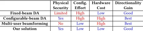
Fixed-beam DA Limited High Low Good
Conigurable-beam DA Yes High High Best
Multi-user beamforming No Low High Best
Our solution Yes Low Low Good
Table 1:Comparing our solution to directional antennas (DA) or beamforming.
APs without directional or multiple antennas. Table 1 compares our solution to its alternatives.
Our work comprises two technical components:First, we de-sign an efective optimization algorithm that optimizes relector 3D shapes for a target wireless coverage. During this process, we represent a relector shape as a parametric model [39] in computer graphics to ensure surface smoothness and in turn the feasibility of 3D fabrication. The shape optimization leverages a 3D wireless modeling to evaluate the efectiveness of a candidate shape and improve the shape iteratively. We guide a Simulated Annealing algorithm [28] using local gradient descent to sample the shape space more eiciently. We also extend our optimization to deal with multiple APs and jointly optimize their relector shapes.Second, we develop an eicient modeling approach that uses 3D ray trac-ing to simulate radio signal propagation and signal’s interaction with objects in a 3D environment. We consider signal’s relection, transmission, and difraction through objects. For APs with multi-ple antennas, we also take into account the antenna location and orientation to trace radio signals accurately in the 3D space.
We 3D print optimized relectors, test them with various Wi-Fi APs (including the latest 802.11ac AP) via signal and throughput measurements in two indoor settings. Our indings are as follows:
• Optimized relectors correctly adjust signal distribution towards the target coverage. Resulting signal strength can decrease by up to 10 dB and increase by 6 dB, leading to throughput diferences from -63.3% to 55.1%;
• Optimized relectors coexist nicely with various Wi-Fi APs in-cluding MIMO APs (e.g., TP-Link AP and Netgear R7000). They allow multiple APs to collaboratively serve a region, or to conine each AP’s coverage to enhance security and reduce interference;
• The optimized relector is relatively easy to place. Its eicacy is not sensitive to slight placement ofsets, tolerating up to 10◦
ofset in orientation and 10 cm ofset in the distance to the AP.
• Given an environment model, our system computes an optimized relector shape in 23 minutes on a laptop (2.2. GHz Intel Core i7). Our work presents a low-cost, secure, and easy-to-conigure ap-proach that can coexist with directional communication via multi-antenna beamforming. Physical relectors regulate signal distribu-tion across regions at the macro level, while beamforming enables iner-grained signal enhancement at individual clients within the coverage. While we use Wi-Fi as an example, our approach can be generalized to other wireless bands (e.g., light, millimeter waves, acoustics). It can improve eiciency of diverse wireless networks in built environments, and potentially help in delivering higher-order services for buildings, e.g., occupancy detection, lighting control.
2
SYSTEM OVERVIEW
Our system takes three inputs: 1) a digitized, simpliied environ-mental model including the main room structure (e.g., walls); 2)
information of wireless APs: their locations, the number of anten-nas, and positions of antennas if they are external antennas; and 3) the target wireless coverage speciied as areas where users aim to strengthen or weaken the received signal strength.
The core of our system is an iterative stochastic optimization process that searches for a 3D relector shape for each AP, so that collectively they achieve the target wireless coverage. Starting from an initial 3D shape and relector position, our algorithm perturbs the current shape and estimates the resulting signal distribution with the new shape. Based on an objective function that measures the quality of a relector shape, it then chooses to accept or re-ject the perturbed shape before moving on to the next iteration. Evaluating the objective function requires a 3D wireless propaga-tion model that predicts the spatial distribupropaga-tion of received signal strength. Our wireless propagation model takes into account the indoor environment and simulates the radio waves interacting with environment objects. The process stabilizes at a inal shape until no further improvement can be made to better match the target.
Finally, we output the shape and placement of the relector, then the user fabricates the optimized relector shape and coats it with a thin metal layer (e.g., aluminum foil) to enhance its ability to relect wireless signals. The fabricated relector is then mounted around the wireless AP to realize the customization of wireless coverage. Next, we describe our optimization of relection shape, followed by wireless propagation modeling and relector fabrication.
3
REFLECTOR SHAPE OPTIMIZATION
We optimize the relector shape, aiming to generate a target wireless coverage for a given environment. We irst present parameterizing the 3D geometry of a relector, followed by our shape optimization procedure, as well as its extension to deal with multiple APs.
3.1
Representing the Relector Shape
To represent a 3D surface, we seek a shape parameterization that can express a large space of feasible shapes and yet entail a low con-trol degrees of freedom for the sake of computational performance. A naive solution is to represent a shape as a triangle mesh and optimize the positions of mesh vertices. However, this approach has a large number of optimization variables (i.e., the positions of mesh vertices). It results into an optimization problem in a high dimensional space, which is rather computationally expensive. Fur-thermore, the resulting shape might not be well-formed and thus cannot be fabricated in practice.
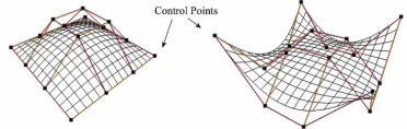
Figure 1:NURBS surface [39] to generate and control a 3D surface using a few (4×4) control points.
curve. By manipulating the knot vector, we can decide whether the curve passes through or passes by certain control points. The size of the knot vector is equal to the number of control points plus the order. The order deines the number of nearby control points that inluence any given point on the curve.
A NURBS surface is calculated as the tensor product of two NURBS curves. Thus, it has two parametric directions (uandv) and two corresponding orders and knot vectors. For our purposes, we predeine its knot vectors and orders and then manipulate its shape by changing positions of the control points. A NURBS surface Ω(u,v)is constructed as:
Ω(u,v)=
l
X
i=1
w
X
j=1
Ri,j(u,v)Pi,j, (1)
with
Ri,j(u,v)= Ni,n
(u)Nj,m(v)wi,j
Pl p=1
Pw
q=1Np,n(u)Nq,m(v)wp,q
as rational basis functions, where we havel×wcontrol pointsPi,j, andwi,j is the corresponding weight.Ni,n(u)is theit hB-spline
basis function of degreen[19]. In our model, a shapeΩis deined byl×wcontrol pointsPi,j. We set their weights as 1, which is a common usage. Figure 1 illustrates two example NURBS surfaces with 4×4 control points, where we lift the center control points to generate a concave shape on the left and then lift the four corner points to generate the shape on the right.
3.2
Optimizing the Relector Shape
To search for the relector shape optimized for a target coverage, we start with a lat plane as the relector shapeΩand then perturbΩ over iterations. In each iteration, we evaluate the efectiveness of a candidate shapeΩby the objective functionF(Ω), whereF(Ω) mea-sures the diference between the desired coverage and the coverage
CΩresulting from relector shapeΩ. We estimateCΩby running the 3D wireless modeling described in Section 4. Speciically, we divide the environment into small cells in uniform size (1 m×1 m in our implementation). We apply the 3D wireless propagation modeling to predict signal strength at each cell’s center. Assuming
M+andM−denote the areas where users aim to strengthen and
weaken signals respectively, we computeF(Ω)as:
F(Ω)= X
i∈M+∪M−
||CT ar дet(i)−CΩ(i)||2, (2)
whereCΩ(i)is the signal strength in dBm at celliafter placing re-lector shapeΩ, andCT ar дet(i)is the target signal strength of celli.
To deriveCT ar дet(i), we irst compute signalC(i), which is the
esti-mated signal strength at celliwhen no relector is placed. We then add/subtractδ, which is the expected signal enhancement/reduction
(a) (b)
Figure 2: (a) shows the objective function F(Ω) as we perturb two control points of the NURBS surface. (b) illustrates our search method. In the(k−1)-th iteration (Ωk−1), we apply gradient descent to seek the local optimumΩ′kand chooseΩ′kas the next candidate.
at celli. To determineδ, we tested diferent materials on their per-formance of signal enhancement and attenuation at distances from 1 to 3 meters. Results (Figure 5) show that the signal change is at most 15 dB. Thus we setδto 15 dB and writeCT ar дet(i)as:
CT ar дet(i)=
C(i)+δ ifi∈M+
C(i)−δ ifi∈M−. (3)
Here we use a cell-dependent target valueCT ar дet(i), rather than a
uniform signal upper and lower bound, becauseCT ar дet(i)deines
an equal range (δ) above or belowC(i). As a result, a given amount of signal enhancement or reduction leads to the same amount of change inF(·), regardless of the cell location. This, however, is no longer guaranteed if a uniform bound is used, because of the quadratic nature ofF(·). Thus,CT ar дet(i)ensures the optimization
process is unbiased across cells. Finally, the optimization process searches forΩ⋆:Ω⋆=argminΩF(Ω), whereΩ⋆is the 3D relector shape that leads to signal distribution best matching the target.
While the optimization problem appears standard, the search space is daunting and many local optimums exist (Figure 2(a)). Sim-ple local search methods such as hill climbing can easily be stuck at local optimums. We need eicient algorithm to identify the global optimal. To achieve this goal, we consider simulated annealing (SA) [28], which allows the iterations to opportunistically escape from the current local search area even if the escape leads to an increase in the objective function. The escape likelihoodpis deter-mined by two parameters in the algorithm: current temperatureT
and the increase in the objective function. SA keeps examining can-didate shapes untilTreaches the minimal temperature (0). When a candidate shapeΩis examined, the current temperature is cooled at a rater. SA acceptsΩifF(Ω)is lower than the previous candi-date. Otherwise, it acceptsΩwith a probabilityp.pis adapted over iterations. In the beginning whenT is higher,pis also higher so SA tends to explore other areas in the shape space. AsTdecreases to 0,papproaches 0 so that it gradually settles at an optimum.
Algorithm 1Shape Optimization 1: initializeΩk,k=0,T=Tmax 2:whileT >Tmi ndo 3: k←k+1 4: F(Ωk−1)←Eq.(2)
5: Ωk←per tur b(Ωk−1)
6: while do
7: ∇F(Ωk)←дet Gr adient(F(Ωk)) 8: λ←дet S t epSize()
9: ifF(Ωk−λ∇F(Ωk))<F(Ωk)then 10: Ωk←Ωk−λ∇F(Ωk)
11: else
12: break
13: end if 14: end while 15: F(Ωk)←Eq.(2) 16: p←e
F(Ωk−1)−F(Ωk)
T
17: ifF(Ωk−1)≥F(Ωk)orr and[0,1]≤pthen
18: Ω⋆
←Ωk 19: end if 20: T←T ·r
21:end while 22:return Ω⋆
functionF(Ωk)atΩk:
∇F(Ωk)= lim
| |dΩk| |→0
F(Ωk+dΩk)−F(Ωk)
dΩk , (4)
wheredΩkis obtained by slightly changing the control points of Ωk. Then we apply backtracking line search to ind an appropriate step sizeλ. Finally we takeΩk−λ∇F(Ωk)asΩkand repeat Eq. (4) until we ind a local optimumΩk′. We takeΩk′ as the candidate instead ofΩkto go over the accept/reject procedure. This method directly iterates from one local minimum to another (Figure 2(b)), and thus is more eicient to approach the global optimum than SA’s random sampling [31]. Algorithm 1 lists the detail.
Accelerating the Search. Each iteration in our search can be time-consuming, because deriving∇F(Ωk)requires altering the positions ofΩk’s control points one by one. The running time of each iteration is linear with the number ofΩk’s control points. To speed up the gradient computation, we leverage the simultaneous perturbation stochastic approximation (SPSA) algorithm [13, 46], which perturbs all parameters (i.e., control points) simultaneously with a random perturbation vector∆to estimate the gradient of each parameter. Thus, it approximates the gradient computation using only two calculations of the objective function, regardless of the parameter dimension (i.e., the number of control points in our problem). Additionally, we run these iterations as parallel threads to further shorten the process. As a result, an iteration take 1.71 seconds on average on a MacBook Pro (2.2 GHz Intel Core i7).
3.3
Extending to Multiple APs
We now extend the above shape optimization to handle multiple APs. We classify APs into two types:1) Collaborative APs: APs that are deployed by the same entity, e.g., a user or an enterprise deploying multiple APs in a home or workplace. These APs collab-oratively serve a region to provide wireless coverage and user’s device automatically connects to the AP with the strongest signal;
2) Non-Collaborative APs: APs that are deployed by diferent enti-ties. Each AP serves users in its own pre-deined coverage region, without the knowledge nor any control of other APs.
For collaborative APs, we jointly optimize their relector shapes so that the resulting signal coverage best matches the target. Here the signal coverage map is deined based on the strongest sig-nal received at a location from all collaborative APs. Thus, let
O ={Ω1, ...,ΩM}denote a set of candidate relector shapes for
Mcollaborative APs, whereΩjis the relector shape for APj. Then
its objective functionF(O)is similar to Eq.(2):
F(O)= X
i∈M+∪M−
||CT ar дet(i)−CO(i)||2, (5)
whereCO(i)is the signal strength at celliafter placing relector
shapesOat all APs.CT ar дet(i)is computed following Eq.(3), but
withC(i)as the signal received at cellifrom the strongest AP. Thus the search is to seek the optimal set of shapesO⋆=argminOF(O). To jointly optimizeMrelectors, we interleave the perturbation of each AP’s relector shape across iterations. Speciically, in an iteration, we perturb only one AP’s relector shape to seek its next candidate shape while ixing other APs’ relector shapes, and then move on to perturbing the next AP’s relector shape in the next iteration. Each iteration of the optimization procedure is similar to Algorithm 1. We omit the algorithm details in the interest of space. For non-collaborative APs, each AP has its own pre-deined coverage region without the knowledge of other APs, thus each AP’s relector shape is optimized separately following Algorithm 1. For non-collaborative APs operating on the same channel, they can interfere with one another if their coverage regions are nearby. The impact of interference can be minimized if the information (e.g., location, relector shape) of other interfering APs is available to the shape optimization algorithm. We can estimate the interference at each cell and consider signal-to-interference ratio (SINR) as the target (Eq. (2)) for shape optimization. We leave it for future work.
4
EFFICIENT 3D WIRELESS MODELING
An essential part of our shape optimization is an eicient modeling that simulates wireless signal propagation in a given environment for evaluating the eicacy of a candidate relector shape. Most ex-isting models either fall far short in modeling accuracy [29, 36], or require expensive measurement or computation overhead. To achieve a better tradeof, we choose 3D ray tracing for its best accuracy [26, 35, 53] and design schemes to speed up its compu-tation. In particular, we choose the Shooting-and-Bouncing Ray (SBR) launching algorithm [21, 30, 43], which launches a number of rays from the transmitter and traces all their possible paths to reach a receiver. Next we describe the key steps of our modeling.
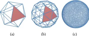
Ray Launching. We model each antenna of a Wi-Fi AP as a signal source3. To achieve accurate ray tracing, rays need to be uniformly spread from the transmitter, i.e., angles between any two adjacent rays are uniform. To do so, we use the geodesic sphere ray launching [51]. A geodesic sphere (Figure 3) is formed by tessellat-ing faces of a regular polyhedron and extrapolattessellat-ing the intersection points on the surface of a sphere [27]. The geodesic vertices pro-vide equivalent angular separation around the entire sphere [43]. Thus, we can place the transmitter at the sphere center and emit a ray to every geodesic vertex on the sphere to guarantee uniform
3More antennas imply more signal sources and thus higher computation overhead in
(a) (b) (c)
Figure 3:Geodesic sphere for uniform ray launching, where a ray is emitted from the sphere center to each geodesic vertex on the sphere. The sphere is generated by tessellating a regular icosahe-dron (a). (b) and (c) show the resulting spheres after tessellating each triangle surface in (a) into 4 and 256 triangles, respectively.
ray launching. In our implementation, we consider tessellating an icosahedron (20 triangular faces and 12 vertices) [54]. To achieve high resolution, we divide each edge intoN=8 segments and thus tessellate each triangle surface intoN2=64 triangles (Figure 3(c)). It leads to 10N2+2 =642 launched rays (i.e., geodesic vertices) with the average radial angular separationθof N1q4π
5√3≈0.1506 rad, where the unit of 4πis steradian [21].
Ray Tracing. We track each ray’s interaction with environmental objects. Given the wavelength of Wi-Fi signals, we consider three types of interactions (Figure 4(a)):transmissions(rays penetrate the objects),relections(a ray is bounced over a smooth surface), and
difractions(a ray hitting an object edge is difracted as a set of rays in a cone shape, Figure 4(b)). To model difraction, we leverage the Uniform Theory of Difraction (UTD) used by the fast-wave acous-tics simulation in computer graphics [52]. It has also been applied in modeling RF propagation in buildings [37]. Similar to [24, 26], we do not consider wave phase as we average signal strengths in each 1 m×1 m cell when evaluating coverage. We do not model other wave phenomena like scattering since they have negligible impact on the resulting signal map [26]. We also do not consider the near-ield efect, since we calculate signal strength at locations at least meters away from the antenna, while the Fraunhofer distance [11] deining the near ield is tens of centimeters in our setting4.
Each type of ray interaction contributes to additional energy loss of a ray, in addition to its signal degradation over distance. To integrate all these contributors, we choose a partition model [9, 26] to calculate each ray’s signal power at a receiver location. The model consists of four parts: 1) the signal degradation over distance, represented by the pathloss exponentα; 2) the relection attenu-ation, which is the product of the relection coeicientβand the number of relections; 3) the transmission attenuation, which is the product of the transmission coeicientγand the number of times that a ray penetrates obstacles; and 4) the difraction attenuation, which is the product of the difraction coeicientλand the num-ber of difractions. We do not consider multiple difractions and relection-difraction [43].
Formally, letPijdenote the power in dBm contributed by theit h
ray ofjt hAP after traveling a distance ofdi to reach a receiver, we
can calculatePijas:
Pij =P0j−10αloд10(di/d0)−βNi,r e f −γ Ni,t r ans
−λNi,di f f −β′Ni′,r e f −γ′Ni′,t r ans,
(6)
4Fraunhofer distance is calculated as2D2/λ, whereDis the largest physical linear
dimension of the antenna andλis the wavelength.
Tx
reception sphere
ray1, transmission
ray3, diffraction
ray2, reflection
Rx
(a) ray interactions
Incident ray
Diffracted rays Edge
θi θd
θi = θd
(b) Uniform theory of difraction
Figure 4:Ray tracing.
whereP0j(in dBm) is the reference power ofjt hAP at distanced0, pathloss exponentαcaptures how quickly the signal degrades over distance,Ni,r e f,Ni,t r ans,Ni,di f f are the number of relections,
transmissions, and difractions that rayiexperiences, respectively. Since the relector surface is designed to be highly relective, we consider diferent transmission and relection coeicients (β′,γ′) for the relector.Ni′,r e f andNi′,t r ans are the number of times rayi
penetrates and is relected by the relector, respectively.
We can adapt the model to various environments easily as param-eters (P0j,α,β,γ,λ,β′,γ′) are calibrated only once. The calibration needs measurements only at a few sampled locations, rather than a site survey. The best-it parameter values are identiied by apply-ing simulated annealapply-ing [26] to minimize modelapply-ing errors. These parameters can then be reused at all locations of an environment.
Ray Reception. Finally to calculate the received signal strength at a receiver location, we sum the power of each ray within the reception zoneZof this receiver. Formally, letPj(in dBm) be the received power from APj, we havePj = 10loд10Pi∈Z10P
j
i/10,
wherePij is the power contributed by rayifrom APjcalculated by Eq. (6). We consider the reception zone as a sphere with radius ofθd/√3 centered at the receiver [42], whereθ is the average radial angular separation between adjacent rays launched from the transmitter, anddis the length of a ray’s propagation path to the receiver. The radius of the reception sphere considers the fact that rays are spread out as they propagate. Figure 4 shows the reception sphere for each ray, where ray2 travels the longest distance to reach receiver and thus has the largest reception sphere.
Speeding Up Ray Tracing. While ofering higher accuracy, ray tracing incurs heavy computation, mainly because of calculating intersections of a large number of rays and triangle meshes5. To speed up the ray tracing process, we index the triangle meshes with a Kd-Tree [12]. We construct a Kd-Tree of the bounding boxes containing these triangle meshes. For each ray, we irst search the tree to identify the bounding boxes that the ray intersects. Only for the triangle meshes in those bounding boxes, we examine the ray-triangle intersection, which avoids many unnecessary intersection tests. For each ray-box and ray-triangle intersection test, we apply prior algorithms [22, 32] to improve the eiciency.
5
REFLECTOR FABRICATION
With the optimized shapeΩ⋆, the last step is to realize it as a physical relector. We representΩ⋆as its corresponding control points of the NURBS surface, calculate the coordinates of each mesh point based on Eq. (1), and store all mesh points in an .obj ile. We
5In our implementation, the indoor model has 107 triangle meshes and the ray tracing
5 10 15 20
1m 2m 3m
Signal enhancement (dB)
Measurement Distance from AP (m) 0.1mm copper
0.1mm silver 0.1mm aluminum 0.25mm aluminum
(a) Signal enhancement
5 10 15 20
1m 2m 3m
Signal attenuation (dB)
Distance from AP (m) 0.1mm copper
0.1mm silver 0.1mm aluminum 0.25mm aluminum
(b) Signal attenuation
Figure 5:Diferent plane relector’s ability to relect and attenuate Wi-Fi signals, at distances from 1 to 3 meters.
edit the .obj ile in Blender, an open-source 3D computer graphics software. We add thickness and export it to a .stl ile for a 3D printer (MakerBot) to print it. Its build volume is 25.2 cm×20 cm×15.0 cm. Overall fabricating a 20 cm×20 cm relector costs no more than $35 (one large spool of MakerBot PLA Filamen).
We add a thin layer of metal to the plastic relector surface because metals have exceedingly high conductivities and thus are efective relectors and attenuators of radio waves [3]. To determine the metal material, we systematically test three types of metal sheets made of silver, copper, and aluminum, which are all 0.1-mm thick. We also test aluminum sheet with 0.25-mm thickness to evaluate the impact of the metal-layer thickness. We attach each metal sheet to a 30 cm×30 cm plastic (the same material used by 3D printers in fabrication) to form the inal relector. We place the relector at the back of an AP to test its ability to relect Wi-Fi signals to a receiver. To test its ability to attenuate signals, we place the relector between the AP and the receiver. For both tests, we vary the distance of the receiver to the AP from 1 m to 3 m.
In Figure 5, we see that copper and aluminum perform similarly in enhancing and attenuating Wi-Fi signals, and silver performs slightly better. Increasing sheet thickness moderately improves its ability to attenuate signals, but not its relection property. Given the lower cost of aluminum and the diiculty of applying a 0.1-mm sheet to an uneven relector surface, we choose to cover the relector surface with a 0.024-mm household aluminum foil.
We also observe that relectors are better at weakening than strengthening Wi-Fi signals, mainly because of Wi-Fi’s wavelength and the energy loss when signals penetrate the relector. When Wi-Fi signals interact with the relector, the signal either penetrates, or is absorbed, or is relected by the relector. Only the relected energy can be directed to strengthen the signal at locations before the relector, while both the relected and the absorbed energy contribute to the signal attenuation at locations behind the relector.
6
EVALUATION
We evaluate our approach by testing optimized relectors in two indoor scenes. We seek to understand its capability in afecting wire-less signal distribution and throughput, implications on enhancing security and reducing interference, its sensitivity to relector place-ment and size, and other performance microbenmarks.
6.1
Experimental Setup
Indoor Scenes. We experiment two indoor scenarios with difer-ent room layouts: (a)workspace scenario: a 19 m×13 m indoor area with a narrow (7.5-m long) hallway connecting a research lab and
two oices; (b)home scenario: a 16 m×12 m area where a spacious lobby (5.8 m×5.1 m) is surrounded by three rooms. Figure 6(a) and Figure 7(a) show their loor maps, respectively. Although rooms are furnished in both scenes, the 3D environment models used in our shape optimization contain only walls and doors (we will evaluate the impact of including furniture in environment models in ğ 6.5). Experiments are conducted during working hours with moving users around (walking, working at their desks, or stand-ing and talkstand-ing to others). For the simplicity and feasibility of the user input, we assume the same material for objects in the envi-ronment. To consider heterogeneous materials, we can adapt the relection, transmission and difraction coeicients in Eq. (6) based on materials, and track what materials a ray has traveled through.
Wi-Fi APs. We use Netgear R7000 (IEEE 802.11ac) as default APs. R7000 has three antennas and operates on both 2.4 GHz and 5 GHz frequency. We conigure it to transmit at 10 mW and collect RSS values at 2.4 GHz band. We also test two other popular APs: Linksys WRT54GL (IEEE 802.11g) and TP-Link WR841N (IEEE 802.11n), both operating on 2.4 GHz frequency and equipped with two external antennas. To minimize interference from external APs, we analyze channel usage status using a mobile app (Wi-Fi Analyzer) and set the AP to operate on the least congested channel (channel 9 in our environment).
Ground Truth Signal Collection. Although our approach does not require exhaustive site survey measurements to compute re-lector shapes, such measurements are necessary for us to evaluate the impact of optimized relectors on signal distribution. To gather signal measurements, we divide each area into 1 m×1 m cells and average received signal strength (RSS) values within each cell. We also sample a few locations (blue circles in Figure 6(a) and Figure 7(a)) to measure the throughput.
To automate RSS measurements in the 3D space, we apply a drone-based method in [55]. We program an AR Drone 2.0 to collect RSS at speciied locations. We reuse drone’s built-in Wi-Fi radio to receive beacons from our AP and record RSS values. To decide the measurement duration per location, we let the drone hover over a location, measure for 1 minute and 10 seconds respectively, and compare the mean and standard deviation of RSS. Results reveal that 10 seconds are suicient for collecting stable RSS statistics.
6.2
Eicacy of Optimized Relector
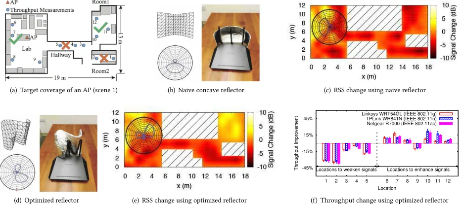
We start by examining the overall eicacy of the optimized relector in a single-AP setting. We consider a target coverage in Figure 6(a), where we mark areas with received signals to be strengthened by ticks and areas with signals to be weakened by crosses. We run our shape optimization algorithm to derive the optimized relector shape, fabricate the relector (20 cm×20 cm in size), and place it around AP’s antennas. Figure 6(d) shows the optimized 3D shape, its estimated radiation pattern, and its placement. The radiation pattern is generated by simulating signal change at one meter away. For this target coverage, an antenna is behind the relector and the others are in front of the relector. We measure changes in the resulting RSS and throughput.
(a) Target coverage of an AP (scene 1) (b) Naive concave relector (c) RSS change using naive relector
(d) Optimized relector (e) RSS change using optimized relector
-45% -15% 15% 45%
1 2 3 4 5 6 7 8 9 10 11 12 Locations to weaken signals Locations to enhance signals
Throughput Improvement
Location
Linksys WRT54GL (IEEE 802.11g) TPLink WR841N (IEEE 802.11n) Netgear R7000 (IEEE 802.11ac)
(f) Throughput change using optimized relector
Figure 6:Eicacy of an optimized relector for achieving a target wireless coverage (a), where areas users aim to strengthen the signal are marked by green ticks and areas to weaken the signal are marked by red crosses. (b) and (c) show a relector in a simple concave shape and its resulting signal change in dB, while (d), (e), and (f) show a relector in optimized shape, and the resulting changes in signal distribution and throughput. The optimized relector shape leads to a signal distribution better matching the target.
the results to that of a naive relector shape (the concave shape used in anecdote experiments, Figure 6(b)). Figure 6(c) and (e) show the RSS change (in dB), where positive numbers indicate signal enhancements and negative numbers indicate signal declines. We observe that the optimized relector correctly adjusts signals in all target areas, weakening signals in the hallway and room2 by 10 dB while strengthening signals in other target areas by 6 dB. It achieves the goal by blocking an antenna that emits signals to the hallway and room2 while relecting the signals of the other two antenna towards room1. The naive relector, however, generates a simple radiation pattern that uniformly weakens signals in all areas in the back of the relector, and thus fails to meet requirements of all target areas. The result demonstrates the necessity and eicacy of our optimization, which considers the indoor layout to customize the relector shape and enables more lexible control.
A side efect of the optimized relector is that in order to weaken signals in the hallway and room2, it also slightly weakens the RSS in the right bottom of the lab. It is a sacriice made by the shape optimization to reach an overall signal distribution better matching the target. As we further analyze signal change at individual cells, 83.1% of cells have their signals correctly strengthened or weakened, demonstrating the overall eicacy of the optimized relector.
Impact on Throughput. We further examine how signal-level changes translate into throughput diferences at clients. We sample a few locations (marked as blue circles in Figure 6(a)) and mea-sure the throughput at those locations before and after placing the relector. In particular, we associate two laptops (MacBook Pro) with our AP. We ix the location of a laptop, while a user holds the other laptop walking around within each location to measure the throughput. We instrument one laptop to transmit 500-MB data to the other using the iperf utility and collect throughput statistics. We repeat the experiment for 10 rounds.
Figure 6(f) shows the percentage of throughput change un-der diferent APs with optimized relectors. We also include er-ror bars covering 90% conidence intervals. Overall throughput in-creases/decreases by up to 22.1%/36.7% in target areas. The through-put improvement at location 8 is small because its RSS is low, re-quiring a larger signal enhancement to switch to higher data rates. The throughput at location 9 slightly decreases because its RSS is slightly weakened by the relector (Figure 6(e)). Most other lo-cations in the lab experience improved throughput. Overall, the optimized relector correctly adjusts throughput for 11 out of 12 lo-cations. The result also shows that our relectors can coexist nicely with MIMO APs (i.e., TP-Link AP and Netgear R7000).
6.3
Multi-AP Settings
We now move on to scenarios with multiple APs. As follows, we consider two types of APs described in ğ 3.3.
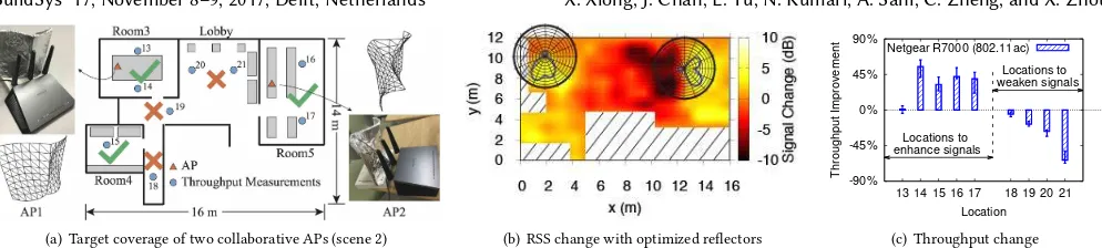
Collaborative APs. To evaluate the eicacy of jointly optimized relectors, we deploy two APs in scene 2 and jointly optimize their relector shapes for a target coverage in Figure 7(a). We measure the signal map before and after placing relectors, where the RSS at a location is the signal from the stronger AP. We plot the signal change in Figure 7(b). The two optimized relectors successfully reduce signal strength in lobby by up to 10 dB and increase signals up to 6dB in room 3, 4 and 56. Overall, 91% of cells have their signals correctly strengthened/weakened. To further examine the impact on resulting bandwidth, we sample 9 locations (blue circles in Figure 7(a)) and plot in Figure 7(c) the throughput change brought by optimized relectors. For 7 out of 9 locations, the throughput changes from -63.3% to 55.1%. Location 13 and 18 experience little change because of their minor signal changes (Figure 7(b)). Overall
6The numbers are slightly diferent from that in Figure 5 since the result here is
(a) Target coverage of two collaborative APs (scene 2) (b) RSS change with optimized relectors
-90% -45% 0% 45%
13 14 15 16 17 18 19 20 21
Locations to enhance signals
Locations to weaken signals
Throughput Improvement
Location Netgear R7000 (802.11ac)
(c) Throughput change
Figure 7:Eicacy of optimized relectors of two collaborative APs to achieve a target wireless coverage. In (a), areas where users aim to strengthen or weaken signals are marked by green ticks and red crosses, respectively. (b) shows the map of resulting signal change in dB. (c) plots the throughput improvement at sampled locations (blue circles in (a)).
(a) Target regions of two non-collaborative APs (scene 1)
0% 30% 60% 90%
1 2 3 4 5 6 7 8 9 Outside
region of AP1 region of AP2Outside
Packet Loss Rate
Location No reflector w/ reflectors
(b) Impact on packet loss rate
0 15 30 45
1 2 3 4 5 6 7 8 9
Region of AP2 Region of AP1
SINR(dB)
Location No reflector w/ reflectors
(c) Impact on SINR
Figure 8:Experiments on eicacy of relectors conining wireless coverage and reducing interference. (a) shows the placement and desired Wi-Fi regions of two APs. (b) plots the packet loss rate change outside the desired region of each AP when optimized relectors are placed. (c) presents relectors’ impact on SINR inside the AP’s desired region.
the signal and throughput changes are notable for the majority of locations, demonstrating the eicacy of our joint optimization.
Non-Collaborative APs. For non-collaborative APs, we aim to conine each AP’s coverage. We examine the implications on secu-rity/privacy and interference reduction with optimized relectors.
1) Implications on Security/Privacy:We set up two Netgear R7000 APs in scene 1 and mark each AP’s coverage region in Figure 8(a). We then fabricate relectors for these APs to conine their coverage. We measure packet loss rates at sampled locations (marked as blue circles) before and after placing relectors. We asso-ciate two laptops (MacBook Pro) with the same AP and instrument a laptop to transmit packets to the other using the iperf utility. Sim-ilarly to [45], we desire packet loss rates above 30% for locations outside an AP’s coverage region, as many TCP and UDP based applications [10, 41] require a packet loss rate below 25%.
Figure 8(b) plots packet loss rates when a receiver outside an AP’s region attempts to connect to this AP. Before placing any relector, all locations have access to both APs. After placing opti-mized relectors, we ind that room2 (location 1 and 2) is unable to access the network of AP1 (50 - 60% packet loss rates), and locations at the lab (location 6, 7 and 8) can not access AP2. This demonstrates that optimized relectors help conine Wi-Fi signal strength in the desired region. We also observe that for some locations outside an AP’s region, packet loss rate does not change much after placing the relector, e.g., the packet loss rate of AP2 at location 9 is nearly 0% with or without the relector. It is because location 9 is relatively close to AP2 and receives a strong signal from AP2 even with the relector. The same holds for location 3, 4, and 5. To address this limitation, we plan in future work to include transmit power as another parameter in our model to control coverage more precisely. 2) Reducing Interference:To quantify the beneit on interfer-ence reduction, we examine Signal to Interferinterfer-ence Noise Ratio
0 2 4
-30 -20 -10 0 10 20 30
Signal Change(dB)
Orientation Offset(degree) Room 1
Room 2
(a) Impact of orientation
0 2 4
0 5 10 15 20 25
Signal Change(dB)
Distance(cm) Room 1 Room 2
(b) Impact of distance
Figure 9:Sensitivity to relector placement ofset.
(SINR) at locations in each AP’s coverage region. We reuse the set-ting in Figure 8(a) and compute the SINR at all locations. Figure 8(c) shows that relectors boost the SINR for most locations by up to 13 dB. The SINR at location 9 barely changes because while AP2’s relector weakens the interference, AP1’s relector also weakens the signal at this location, resulting into little change in its SINR.
6.4
Relector Placement and Size
In addition to the relector shape, the relector placement and size can also afect relector’s eicacy. Next we examine system’s sensi-tivity to these factors. In following experiments, we use the opti-mized relector in Figure 6(d) as an example.
Placement Ofset. We irst study the impact of orientation ofset, which can occur during manual placement. In the experiment, the relector (20 cm×20 cm) faces room1 and room2 to enhance sig-nals, which corresponds to the 0◦orientation ofset. We rotate the relector from−30◦to 30◦in a counterclockwise manner with 5◦
interval. We then plot the average signal enhancement of interested locations in room1 and room2 in Figure 9(a). During the experiment, we observe some large signal variation at certain locations (location 10) when the orientation ofset is within 10◦, but the variation is
0 0.2 0.4 0.6 0.8 1
0 2 4 6 8 10 12
CDF
Error (dBm) 3D w/ furniture 3D w/o furniture 2D w/ furniture 2D w/o furniture
(a) no relector
0 0.2 0.4 0.6 0.8 1
0 2 4 6 8 10 12 14 16
CDF
Error (dBm) 3D w/ furniture 3D w/o furniture 2D w/ furniture 2D w/o furniture
(b) concave relector
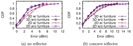
Figure 10:Accuracy of 3D wireless propagation modeling, in com-parison to the 2D modeling in prior work [16].
We then examine how the distance between the relector and AP afects the performance. We ix the relector’s orientation, vary its distance from 0 cm to 25 cm with 5-cm interval, and plot the average signal enhancement at room1 and room2 in Figure 9(b). We observe that ofsets within 10 cm have negligible impact. Once the distance is above 10 cm, the signal enhancement starts to decrease. It is because as signals travel, they are further spread out with atten-uated strength. Thus, a relector further away from the AP relects fewer signals and is less efective in afecting signal distribution.
Relector Size. We also study the impact of relector size on relector’s ability to adjust signal distribution. A larger relector relects more signals and can be more efective, however its fabri-cation is harder and more costly. We aim to seek a proper size to achieve a good tradeof. We fabricate the relector in two sizes: 20 cm×20 cm and 40 cm×40 cm. Given that the height and width of all our APs are roughly 20 cm, a 20 cm×20 cm relector can cover all antennas. We place each relector around the AP and measure the resulting RSS change at room1 and room2. As we compare the mean RSS change and the standard deviation for these two sizes, we observe negligible diference, indicating as long as the relector covers all antennas, it needs not to be larger. This observation can be a guideline for determining relector size for APs in other sizes.
6.5
Microbenchmarks
Finally, we examine the accuracy of our 3D wireless modeling and overall running time of the shape optimization.
Accuracy of 3D Wireless Modeling. Using scene 1 as an ex-ample, Figure 10 (a) and (b) plot CDFs of absolute RSS errors of our 3D wireless model (described in ğ 4), using measured RSS as ground truth. Figure 10 (a) is the result without any relector, while Figure 10 (b) is for a concave shaped relector placed around the AP. Overall the mean RSS error of 3D wireless modeling is 3 dBm. Furthermore, we compare our 3D modeling to the 2D modeling in a prior work [16]. We observe that 3D modeling notably lowers the tail of RSS errors. The maximal error of 2D modeling is 11 dBm and 16 dBm, with and without relector respectively, while they are 8 dBm and 12 dBm for 3D modeling. 3D modeling outperforms 2D modeling because of more accurate characterization of signal interaction in the third dimension. We also include the results when 2D/3D wireless modeling uses a iner-grained environment model that includes main furniture (e.g., desks, sofas). We observe that for both 2D and 3D modeling, adding furniture leads to negligible dif-ference in resulting accuracy in both scenarios. The results indicate that coarse-grained 3D environmental models are suicient.
Running Time. We run our shape optimization algorithm on a MacBook Pro (2.2 GHz Intel Core i7) and record the time to generate
an optimized shape for various target coverage requirements. We observe that the algorithm stabilizes after 23 minutes on average. We further look into efectiveness of our speedup schemes: the Kd-tree used to speed up wireless modeling, the SPSA algorithm and multiple threads to speed up the search for optimized shape. Table 2 lists the running time of the optimization process when using either no speedup scheme, or only one speedup scheme, or all of them. Having 107 triangle meshes and 10K rays in the ray tracing model, we see that the Kd-tree accelerate around 1.6 times. For a complex model that has thousands of triangle meshes, the speedup of Kd-tree can be up to tens of times. Theoretically SPSA can reduce tens of time to calculate the gradient when we have 3×5 control points, however it only speeds up roughly 1.5 times, because the search for appropriate step size is another bottleneck. Multiple threads accelerate nearly 4 times. Together, they reduce the average running time from 207 minutes to 23 minutes.
Scheme No SPSA Kd-tree Threads Full
speedup only only only speedup
Time (minutes) 207 141 128 48 23
Table 2:Running time of our shape optimization with and without speedup schemes (SPSA, Kd-Tree, and multiple threads).
7
RELATED WORK
Coniguring Wireless Coverage. Prior works have optimized AP placement to improve signal reception in certain areas [35]. However, moving the AP to enhance one area would result into the decline of signal strength in other areas. Thus, such methods are constrained in its lexibility. Another method is to use directional APs to conine wireless coverage to a speciied region [45]. However, this method needs multiple costly directional APs. Our approach works with a single AP without directional antennas.
As for the use of relectors, recent work [20, 49, 50] has studied reusing walls to relect radio waves and control signal propagation. This method, however, relies on smart walls made of special mate-rials and requires infrastructure-level changes. Similarly, a latest work [23] examined placing multiple metal plates in the environ-ment to enhance wireless performance of a single AP. This approach also requires nontrivial changes in the environment by installing relectors likely in large sizes. In contrast, our approach uses only a small relector at the AP, is applicable in any environment, and supports multiple APs. Additionally, [23] optimizes relector loca-tions, whereas our work optimizes relector shape. Another prior work [16] studied the feasibility of applying fabricated relector to control wireless coverage. We advance this prior work in multiple fronts: a more sophisticated shape model, a more eicient shape optimization and extension to multiple APs, 3D wireless modeling, and extensive indoor experiments with optimized relectors.
Directional antennas often rely on multi-antenna beamforming, which electronically adjusts an array of omni-antennas to form narrow beams and maximize the signal strength for one or multiple users [5, 44]. Despite its superior performance, it has three main limitations. First, it cannot provide physical security, as it only enhances client’s signal reception and cannot take into account client’s location information (i.e., whether the client is inside the authorized location or not). As a result, it can end up forming a beam towards an attacker outside the authorized area. Second, it is more costly than our solution as it requires multiple antennas, each with a separate RF chain. Finally, it imposes expensive measurement overhead by collecting real-time Channel State Information (CSI).
8
CONCLUSION AND FUTURE WORK
We studied the design of a low-cost, 3D-fabricated relector to customize wireless coverage. We demonstrated the eicacy of opti-mized relectors with relector prototypes and indoor experiments. We summarize the limitations of our study and plans for future work.First, our current relectors are in static shapes. Thus, upon substantial changes in the environment (e.g., removal/addition of walls), the relector shape needs to be re-calculated and fabricated. Minor furniture changes have minimal impact on the resulting coverage, as shown in Figure 10, thus not requiring to replace the relector. In the future, we will study relectors made of trans-formable materials, enabling the relector to automatically adapt its shape upon major changes.Second,the wavelength of Wi-Fi signals limits relector’s ability to relect and block signals (Fig-ure 5). Thus, changes on RSS and throughput have been moderate. Moving forward, we will examine higher frequency bands such as millimeter waves and visible light, where relectors can block and relect signals more efectively and cause more signiicant change in signal distribution.Finally, we will explore augmenting directional antennas with optimized relectors and analyze their interplay.
REFERENCES
[5] 802.11ac In-Depth. White Paper, Aruba Networks.
[6] Phocus array. http://www.idelity-comtech.com/products/phocus-array/. [7] Shapeways. https://www.shapeways.com/.
[8] Amiri Sani, A., Zhong, L., and Sabharwal, A.Directional antenna diversity for mobile devices: Characterizations and solutions. InProc. of MobiCom(2010). [9] Bahl, P., and Padmanabhan, V. N. RADAR: An in-building RF-based user
location and tracking system. InProc. of INFOCOM(2000).
[10] Balakrishnan, H., et al.A Comparison of Mechanisms for Improving TCP Performance over Wireless Links.IEEE/ACM Trans. Netw. 5, 6 (1997), 756ś769. [11] Balanis, C. A.Antenna theory: analysis and design. John Wiley & Sons, 2016. [12] Bentley, J. L.Multidimensional binary search trees used for associative searching.
Communications of ACM 18, 9 (Sept. 1975), 509ś517.
[13] Bhatnagar, S., Prasad, H. L., and Prashanth, L. A. Stochastic Recursive Algorithms for Optimization: Simultaneous Perturbation Methods. Springer, 2013. [14] Blanco, M., et al.On the efectiveness of switched beam antennas in indoor
environments. InProc. of PAM(2008).
[15] Buettner, M., et al.A phased array antenna testbed for evaluating directionality in wireless networks. InProc. of MobiEval(2007).
[16] Chan, J., Zheng, C., and Zhou, X.3D Printing Your Wireless Coverage. InProc. of HotWireless(2015).
[17] Chen, J., Bautembach, D., and Izadi, S.Scalable real-time volumetric surface reconstruction. InProc. of SIGGRAPH(2013).
[18] Cottrell, J. A., Hughes, T. J., and Bazilevs, Y.Isogeometric analysis: toward integration of CAD and FEA. John Wiley & Sons, 2009.
[19] De Boor, C., De Boor, C., De Boor, C., and De Boor, C.A practical guide to splines, vol. 27. Springer-Verlag New York, 1978.
[20] Dupre, M., et al. Recycling radio waves with smart walls. InInternational Conference on Metamaterials, Photonic Crystals and Plasmonics(2015). [21] Durgin, G., Patwari, N., and Rappaport, T. S.An advanced 3D ray launching
method for wireless propagation prediction. InProc. of VTC(1997). [22] Glassner, A. S.An introduction to ray tracing. Elsevier, 1989.
[23] Han, S., and Shin, K. G.Enhancing Wireless Performance Using Relectors. In
Proc. of INFOCOM(2017).
[24] Hassan-Ali, M., and Pahlavan, K. A new statistical model for site-speciic indoor radio propagation prediction based on geometric optics and geometric probability.IEEE transactions on Wireless Communications 1, 1 (2002), 112ś124. [25] Izadi, S., et al.KinectFusion: Real-time 3D Reconstruction and Interaction Using
a Moving Depth Camera. InProc. of UIST(2011).
[26] Ji, Y., Biaz, S., Pandey, S., and Agrawal, P.ARIADNE: a dynamic indoor signal map construction and localization system. InProc. of MobiSys(2006). [27] Kenner, H.Geodesic math and how to use it. Univ of California Press, 1976. [28] Kirkpatrick, S. Optimization by simulated annealing: Quantitative studies.
Journal of statistical physics 34, 5-6 (1984), 975ś986.
[29] Kotz, D., et al.Experimental evaluation of wireless simulation assumptions. In
Proc. of MSWiM(2004).
[30] Ling, H., et al.Shooting and bouncing rays: Calculating the rcs of an arbitrarily shaped cavity.IEEE Transactions on Antennas and Propagation 37, 2 (1989), 194ś 205.
[31] Martin, O. C., and Otto, S. W. Combining simulated annealing with local search heuristics.Annals of Operations Research 63, 1 (1996), 57ś75.
[32] Möller, T., and Trumbore, B.Fast, minimum storage ray/triangle intersection. InACM SIGGRAPH 2005 Courses(2005), ACM, p. 7.
[33] Navda, V., et al. MobiSteer: using steerable beam directional antenna for vehicular network access. InProc. of MobiSys(2007).
[34] Niculescu, D., and Nath, B.Vor base stations for indoor 802.11 positioning. In
Proc. of MobiCom(2004), ACM.
[35] Panjwani, M. A., et al.Interactive computation of coverage regions for wire-less communication in multiloored indoor environments. Selected Areas in Communications, IEEE Journal on 14, 3 (1996), 420ś430.
[36] Phillips, C., Sicker, D., and Grunwald, D.Bounding the error of path loss models. InProc. of DySPAN(2011).
[37] Rajkumar, A., et al.Predicting RF coverage in large environments using ray-beam tracing and partitioning tree represented geometry.Wireless Networks 2, 2 (1996), 143ś154.
[38] Ramachandran, K., et al.R2D2: Regulating Beam Shape and Rate As Direc-tionality Meets Diversity. InProc. of MobiSys(2009).
[39] Rogers, D. F.An introduction to NURBS: with historical perspective. Elsevier, 2000. [40] Sankar, A., and Seitz, S.Capturing indoor scenes with smartphones. InProc.
of UIST(2012).
[41] Sat, B., and Wah, B. W.Analysis and evaluation of the Skype and Google-talk VoIP systems. InIEEE International Conference on Multimedia and Expo.(2006). [42] Schaubach, K. R., et al.A ray tracing method for predicting path loss and delay
spread in microcellular environments. InProc. of VTC(1992).
[43] Seidel, S. Y., and Rappaport, T. S. Site-speciic propagation prediction for wireless in-building personal communication system design.Vehicular Technology, IEEE Transactions on 43, 4 (1994), 879ś891.
[44] Shepard, C., et al.Argos: Practical many-antenna base stations. InProc. of MobiCom(2012).
[45] Sheth, A., Seshan, S., and Wetherall, D.Geo-fencing: Conining Wi-Fi cover-age to physical boundaries. InPervasive Computing. Springer, 2009, pp. 274ś290. [46] Spall, J. C.Multivariate stochastic approximation using a simultaneous pertur-bation gradient approximation.IEEE Transactions on Automatic Control 37, 3 (1992), 332ś341.
[47] Subramanian, A. P., et al.A measurement study of inter-vehicular communi-cation using steerable beam directional antenna. InProc. of VANET(2008). [48] Subramanian, A. P., et al.Experimental characterization of sectorized antennas
in dense 802.11 wireless mesh networks. InProc. of MobiHoc(2009).
[49] Subrt, L., and Pechac, P.Controlling propagation environments using intelli-gent walls. InEuropean Conference on Antennas and Propagation(2012). [50] Subrt, L., and Pechac, P.Intelligent walls as autonomous parts of smart indoor
environments.IET Communications 6, 8 (May 2012), 1004ś1010.
[51] Tan, S., and Tan, H.Modelling and measurements of channel impulse response for an indoor wireless communication system. InMicrowaves, Antennas and Propagation, IEE Proceedings(1995), vol. 142, IET, p. 405.
[52] Tsingos, N., et al.Modeling acoustics in virtual environments using the uniform theory of difraction. InProc. of SIGGRAPH(2001).
[53] Valenzuela, R. A.A ray tracing approach to predicting indoor wireless trans-mission. InProc. of VTC(1993).
[54] Wenninger, M. J.Spherical models, vol. 3. Courier Corporation, 1979. [55] Yu, E., Xiong, X., and Zhou, X.Automating 3D Wireless Measurements with