RISK MANAGEMENT USING VAR SIMULATION WITH APPLICATIONS TO BUCHAREST STOCK EXCHANGE
Alin V. Ros¸ca
Abstract. In a recent paper, we have proposed and analyzed, from a theoretical point of view, a multidimensional stock market model (see [?]). In this paper, we construct a portfolio of stocks for a particular case of this market model. We introduce the Value at Risk, as a powerful tool for managing risks, which follow from holding such a portfolio. We present a mathematical calculation of Value at Risk for our market model. Using this mathematical framework, we develop Monte Carlo, Quasi-Monte Carlo and Mixed Monte Carlo and Quasi-Monte Carlo algorithms for the estimation of Value at Risk. We apply the developed methods to portfolios from Bucharest Stock Exchange.
2000 Mathematics Subject Classification: 11K36, 65C05, 91B28, 91B30, 91B70.
Keywords and phrases: Value at Risk, Stock Market, Monte Carlo method, Quasi-Monte Carlo method, Mixed Monte Carlo and Quasi-Monte Carlo Method.
1. Introduction
In a recent paper (see [9]), we have introduced a multidimensional stock market model and analyzed some important features of it. We have consid-ered n stock prices Si(t), i = 1, n, driven by a multidimensional Brownian motion process B(t) = (B1(t), B2(t), . . . , Bn(t))0≤t≤T on some probability space (Ω,F,P), together with the filtration generated by B(t), denoted by
dS1(t) = S1(t)[µ1(t)dt+σ1(t)dB1(t)], (1)
dSi(t) = Si(t)[µi(t)dt+λσi(t)dB1(t) +
√
1−λ2σi(t)dBi(t)], i= 2, n,(2) whereλis a real parameter, such that−1≤λ≤1 andσ(t) = (σ1(t), . . . , σn(t))>
0.
In this paper, we assume that λ = 0. We therefore get the following market model:
dSi(t) = Si(t)[µidt+σidBi(t)], i= 1, n, (3) where the drifts µi, i= 1, n, and the volatilities σi, i= 1, n, are assumed to be constant over time.
In what follows, we consider a portfolio consisting ofnrisky assets, which, in our case, are then stocks defined in (3). If we denote by pi, i= 1, n, the number of positions we hold on asset i, i = 1, n, then we can define the portfolio value at time t as
V(t) = n
X
i=1
piSi(t). (4)
Holding such a portfolio of stocks is a risky business due the market fluctuations. As we can expect huge losses from having a portfolio, we need a powerful tool to measure financial risks. Value at Risk (VaR) is such a tool for managing risk in financial institutions. VaR traces his roots from the great financial disasters from early 1990s. The valuable lesson that we learned was that poor supervision and risk management can lead to huge losses in tens of millions of dollars. The VaR history is closely connected with the name of the Investment Bank J.P. Morgan. Its president Dennis Weatherstone, in intention to evaluate the total risk his firm is exposed to, asked to his directors to present him daily a briefing on the financial risk of the company. RiskMetrics Department developed such a risk measure, widely used today among financial institutions, which they called Value at Risk (VaR).
1 in 100 chance for a loss grater than 10000 to occur any single day. VaR is a very useful number, as it translates all the complicated market risk factors into a single number, in a currency, which everybody can understand.
As our portfolio is composed only from shares of stocks, it is important to make the following remark on the market model. The process B(t) is the Brownian motion observed for the assets in the market under the measureP, induced by the market. In [9], we defined a risk-neutral probability measure
b
P and an n-dimensional Brownian motion under this risk-neutral probabil-ity measure, denoted by Bb(t) = (Bb1(t), . . . ,Bbn(t)). Using this new defined Brownian motion, the stock price dynamics can be expressed as
dSi =Si(rdt+σidBbi), i= 1, n, (5)
whereris the risk-free rate. It is important to note that the risk-free interest rate is used only with option pricing. The future values of the stocks should be modelled usingµi, i= 1, n, and hence, the market model (3). The param-eter µi is replaced with the risk-free rate r, only in risk-neutral valuation of options. However, we are not trying to create a martingale, but model the future behavior of our portfolio. This is true for Value at Risk models, where we are interested in the future state of the portfolio, not in the present value. Hence, in our Monte Carlo, Quasi-Monte Carlo and Mixed Monte Carlo and Quasi-Monte Carlo simulations, we are going to simulate the real prices of stocks, described in relations (3).
The remaining part of the paper is organized as follows. In Section 2, we present a detailed mathematical calculation of Value at Risk for our market model. Using this mathematical framework, we develop Monte Carlo (MC), Quasi-Monte Carlo (QMC) and Mixed MC and QMC algorithms for estima-tion of Value at Risk. In Secestima-tion 3, we apply the developed methods to two portfolios of stocks from Bucharest Stock Exchange.
2. Monte Carlo Simulation of VaR
There are a variety of methods for computing Value at Risk. Three of them are shortly summarized bellow:
1. Delta-gamma approximation
efficient and easiest to implement. However, it gives a poor estimation for portfolios containing assets with highly non-linear response to risk factors.
2. Historical simulation
Historical Simulation (see [3]) takes a portfolio of assets at a particular point in time and revalues the portfolio a number of times, using a his-tory of prices for the assets in the portfolio. The portfolio revaluations produce a distribution of profit and losses, which can be examined in order to determine the VaR, with a chosen level of confidence. The main criticism of this approach is the assumption that the past can predict the future accurately. This method also relies heavily on the time horizon that is used to capture historical data.
3. Monte Carlo simulation
Monte Carlo simulation (see [1], [3] and [8]) is a good alternative to the above two methods because it can handle any non-linear portfolios and can accommodate any type of distribution of risk factors. This ap-proach simulates possible price paths, for each of the assets, and values the portfolio. After many simulations, VAR can be calculated directly from the simulated distribution of portfolio value change. However, this method is computationally intensive.
In this paper, we focus on the last method: MC simulation. We will also use the methods of QMC and Mixed MC and QMC to calculate VaR estimations.
The SDE equation (3) can be solved using Ito’s theorem (see [10]). Ones obtains
Si(t) = Si(0)e(µi−21σ2i)t+σiBi(t), i= 1, n. (6) This process is called a Geometric Brownian Motion (see [6]). If we want to simulate this stochastic process, then the stock price at timet is given by
Si(t) =Si(0)e(µi−12σi2)t+σi
√
tx(i), i= 1, n, (7) wherex(i)∈N(0,1), i= 1, n, are standard normal random variables andt is the holding time.
that contains the initial values of the stocks. Let σ = (σ1, σn, . . . , σn)T be the volatility vector and µ = (µ1, µ2, . . . , µn)T the drift vector. With these notations, we can rewrite relations (7) in matrix form, as follows:
S(t) = S(0)e(µ−12σ2)t+σ
√
t.∗x, (8)
where the symbol .∗ is used for element by element multiplication and x = (x(1), x(2), . . . , x(n))T is a vector of standard normal variables.
Clearly, if the stocks Si, i = 1, n, are all independent, the collection of stocks can be generated directly, using formula (8). But instead of using
n independent Wiener processes Bi(t), to represent the returns, the market model requires correlated underlying processes. This is an important as-sumption, since in practice, the stock prices from the market are in general correlated.
Let us consider the correlated processes Z1, Z2, . . . , Zn, with the correla-tion matrix C = (ρij)i,j=1,n. We also consider the corresponding covariance matrix Σ. Hence, we are given with
dSi =Si(µidt+σidZi), i= 1, n, (9)
where Zi, i = 1, n, are correlated Brownian motions, with correlation ma-trix C. As a whole, the trends will be apparent, since the processes Zi are correlated according to matrix C.
We rewrite the SDE from (9) in the following form:
dSi =Si
µidt+ n
X
j=1
σijdBj
, i= 1, n. (10)
Our objective is to determine the matrixA= (σi,j)i,j=1,n, such thatAAT = Σ. Proposition 1 If V is an n-dimensional diagonal matrix such that (V)ii=
σi, i = 1, n, and AAT = Σ, then there is a lower triangular matrix L, such
that A=V L.
Proof. BecauseC is a correlation matrix, it follows that it is a symmetric, positive definite matrix. Hence, it has a Cholesky decomposition of the form C =LLT, where L is a lower triangular matrix. We have
AAT = Σ =V CV =V LLTV =V L(V L)T.
From Proposition 1, we obtain
dSi =Si(µidt+σidZi) =Si
µidt+σi i
X
j=1
lijdBj
, i= 1, n, (11)
where (lij)i,j=1,n are the components of the lower triangular matrix L. Hence, in order to capture the correlations among the stocks, we will replace relation (8) with
S(t) =S(0)e(µ−12V σ)t+V Lx
√
t. (12)
If the value of the portfolio at time t is V(t), the holding period is ∆t, and the value of the portfolio at time t+ ∆t is V(t+ ∆t), then the loss in the portfolio value is defined as
Loss=V(t)−V(t+ ∆t). (13)
Having defined the Loss random variable, we present the Value at Risk definition.
Definition 2 (Value at Risk) For a given probability α, the VaR, denoted by δα, is defined by the following relation:
P(Loss≥δα) = α. (14)
Typically, the interval ∆tis fixed to one day or two weeks, and the confidence level α is close to zero, often α = 0.01 or α = 0.05. In the statistical termi-nology, VaR is nothing but the (1−α)’th quantile of the Loss distribution. In what follows, we present the mathematical framework for VaR estima-tion, based on MC method. The relation (14) can be written as
1−P(Loss < δα) = α, (15)
or
F(δα) = 1−α =β, (16) where F denotes the (unknown) cumulative distribution function (cdf) of random variable Loss. The VaR can be expressed in terms of the inverse cdf, as follows:
For a given y, the cdf F(y) can be expressed as an expectation
F(y) = E[1{Loss≤y}] =E[1{V(0)−V(t)≤y}]
= E[1{V(0)−Pni=1piSi(t)≤y}] = E[1
{V(0)−Pni=1piSi(0)e
(µi−12σ2i)t+σi √
tPij=1lij xj
≤y}],
where 1{·} is an indicator function, which returns 1 when the relation {·} is true and 0 otherwise.
We denote byf(x(1), . . . , x(n)) the term1
{V(0)−Pni=1piSi(0)e
(µi−12σi2)t+σi √
tPij=1lij xj
≤y} in the last equality.
It follows that
F(y) =
Z
Rn
f(x(1), . . . , x(n))dΦ(x(1), . . . , x(n)) = I, (18) where Φ(x(1), . . . , x(n)) is a distribution function onRn, which can be factored Φ(x(1), . . . , x(n)) = Ψ1(x(1))·. . .·Ψn(x(n)), and Ψi(x(i)), i = 1, n, represents the standard normal cumulative distribution function, denoted by Ψ. We have denoted the last integral by I.
Using the MC method, I is estimated by sums of the form
ˆ
IKM C = 1
K
K
X
i=1
f(x(1)i , . . . , x(n)i ), (19)
wherexi = (x(1)i , . . . , x (n)
i ),i≥1, are independent identically distributed ran-dom points on Rn, with the common distribution function Φ(x(1), . . . , x(n)). Another representation of this estimation, in terms of the Lossdistribution, is
ˆ
IK = 1
K
K
X
i=1
1{Lossi≤y}, (20) where{Lossi, i= 1, K}are samples from the Lossdistribution. Sorting the samples {Lossi, i= 1, K} in increasing order, we obtain
Then the corresponding sample cumulative distribution function is
FK(y) =
0 if y < Loss(1) i
K if Loss(i)≤y < Loss(i+1), 1 if y ≥Loss(K)
i= 1, . . . , K −1. (22)
From relations (19), (20) and (22), we immediately deduce thaty=Loss([Kβ]) gives FK(y) = β, which satisfies the definition of VaR.
The algorithm which generates VaR is presented next.
Algorithm 3 VaR Generation by Monte Carlo Simulation Method
Input data: The initial stock prices vector S(0) = (S1(0), . . . , Sn(0))T, the horizont time t, the number of simulations K and the confidence level α.
Step 1.
for i= 1, . . . , K do
1.1. Generate a random point xi = (x(1)i , . . . , x (n)
i )T onRn,
with independent identically distributed components, each compo-nent having the common distribution function Ψ.
1.2. Generate the stock prices at time t, using formula (12)
Si(t) =S(0)e(µ−12σ2)t+σ
√
t.∗xi,
(23) where Si(t) = (Si,1(t), . . . , Si,n(t))T.
1.3. Determine the portfolio value at time t, using formula (4)
Vi(t) = n
X
l=1
plSi,l(t).
1.4. Determine the Loss distribution sample as
Lossi(t) = V(0)−Vi(t),
where V(0) is the value of the portfolio at initial time. end for
Step 2. Sort the vector Loss = (Loss1(t), . . . , LossK(t)) in ascending order, i.e.
In order to generate a point xi from Step 1.1, we proceed as follows. We first generate a random point ωi = (ω
(1)
i , . . . , ω (n)
i ), where ω (l)
i is uniformly distributed on [0,1], for each l = 1, . . . , n. Then, for each component ω(l)i ,
l = 1, . . . , n, we apply the inversion method and obtain that Ψ−1 l (ω
(l) i ) =x
(l) i is a random point with the distribution function Ψ.
A similar algorithm can be obtained for the QMC simulation method. First, we have to transform the integration domain to [0,1]n. For this, we use the substitution Ψ−i 1(z(i)) =x(i), i= 1, n, and we obtain
I =
Z
Rn
f(x(1), . . . , x(n))dΨ1(x(1))·. . .·dΨn(x(n)) =
Z
[0,1]n
f(Ψ−11(z(1)), . . . ,Ψn−1(z(n)))dz(1). . . dz(n)
=
Z
[0,1]n
g(z(1), . . . , z(n))dz(1). . . dz(n).
In the last equality, we have denoted
f(Ψ−11(z(1)), . . . ,Ψn−1(z(n)))byg(z(1), . . . , z(n)).
Using the QMC method, the integral I is estimated by sums of the form ˆ
IKQM C = 1
K
K
X
i=1
g(z(1)i , . . . , zi(n)), (24)
where (zi)i≥1 = (zi(1), . . . , z (n)
i )i≥1 is a low-discrepancy sequence on [0,1]n. If we replace in Step 1.1 of the Algorithm (3) the random points xi, i = 1, K, with the low-discrepancy sequence (zi)i≥1 = (zi(1), . . . , z
(n)
i )i≥1 on [0,1]n, and the points xi, i= 1, K, from formula (23) with
(vi)i≥1 = (Ψ−11(z (1)
i ), . . . ,Ψ− 1 n (z
(n) i ))i≥1, then we obtain a QMC Algorithm.
During our experiments, we employed as low-discrepancy sequences on [0,1]n the Halton sequences (see [2] and [5]).
The Mixed MC and QMC method gives the following estimate: ˆ
IKM IX = 1
K
K
X
i=1
where (mi)i≥1 = (qi, zi)i≥1 is ann-dimensionalmixed sequence on [0,1]n (see [7]). First, we generate a low-discrepancy sequence (qi)i≥1, on [0,1]d, then we generate the independent and identically distributed random pointszi, i≥1, on [0,1]n−d. Finally, we concatenateq
i andzi, for each i≥1, and we get our mixed sequence on [0,1]n.
In our experiments, we used as low-discrepancy sequences on [0,1]d for the mixed sequences, the Halton sequences (see [2] and [5]).
If we replace in Step 1.1 of the Algorithm (3) the random points xi, i= 1, K, with the mixed sequence (mi)i≥1 = (qi, zi)i≥1 on [0,1]n, and the points
xi, i= 1, K, from formula (23) with (vi)i≥1 = (Ψ−11(q
(1) i ),Ψ−
1 d (q
(d) i ),Ψ−
1 d+1(z
(d+1)
i ). . . ,Ψ− 1 n (z
(n) i ))i≥1, then we obtain a Mixed MC and QMC algorithm.
3. Application of VaR to portfolios from Bucharest Stock Exchange
In this section, we determine Value at Risk for two portfolios of stocks from Bucharest Stock Exchange. First, we estimate the market model pa-rameters vectors: the drift vector µ and the volatility vector σ. Then, we estimate the correlation matrix C. All the estimations are obtained based on the log-returns series calculated as follows. For each stockSi, i= 1, n, the
j-th entry of the return serie Ri, i= 1, n, is
Rji = log
Si(tj+1) Si(tj)
tj+1−tj
, j = 1, M−1, (26)
where M is the number of observations of each of the stock price series. The data used for our estimations are the stock prices from 15.08.2007 until 8.02.2008. The closing prices for each stock are on daily base and can be obtained freely from the internet site of the Bucharest Stock Exchange,
www.bvb.ro.
We denote by V aRM C, V aRQM C and V aRM IX the outputs of our MC, QMC and Mixed MC and QMC algorithms, respectively. The estimations
V aRM C and V aRM IX are calculated as an average of m simulation runs
V aRM C(M IX) = 1
m
m
X
i=1
V aRM C(M IXi ). (27) We also give the sample standard deviation
s= 1
m−1
m
X
i=1
V aRM C(M IXi )−V aRM C(M IX)2
1 2
, (28)
whereV aRM C(M IX)i represents the estimate from runi,i= 1, m. We use the sample standard deviation to analyze the variance reduction effects. We fix the number of independent runs to m = 10.
3.1. VaR estimation for Portfolio 1
We assume that Portfolio 1, denoted by Π1, contains the stocks of two companies: BANCA TRANSILVANIA S.A. (Symbol TLV) and BRD - Groupe Societe Generale S.A. (Symbol BRD), two of the most liquid companies of the Bucharest Stock Exchange market. We hold 150 shares of each company. The parameters of the stock market model are estimated using Matlab built-in functions and are given bellow:
i 1(TLV) 2(BRD)
Si(0) 0.89 28.20
µi 0.0016 0.0036
[image:11.612.217.363.435.500.2]σi 0.0200 0.0235
Table 1: Parameters of Portfolio Π1. The estimated correlation matrix is
C =
1 0.6964 0.6964 1
.
We consider d= 1 for the Mixed estimate (25).
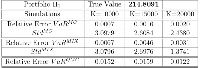
Portfolio Π1 True Value 214.8091
Simulations K=10000 K=15000 K=20000 Relative Error V aRM C 0.0007 0.0016 0.0020
StdM C 3.0979 2.6084 2.4380
Relative Error V aRM IX 0.0067 0.0046 0.0031
StdM IX 3.0796 2.6976 1.3741
[image:12.612.122.457.89.204.2]Relative Error V aRQM C 0.0152 0.0159 0.0122 Table 2: 1-day VaR simulation results.
Portfolio Π1 True Value 568.2147
Simulations K=10000 K=15000 K=20000 Relative Error V aRM C 0.0079 0.0071 0.0017
StdM C 10.1200 9.5613 8.7312
Relative Error V aRM IX 0.0046 0.0001 0.0081
StdM IX 10.8072 7.5239 7.0556
Relative Error V aRQM C 0.0110 0.0110 0.0076 Table 3: 10-day VaR simulation results.
We see that in all methods, the sample standard deviationStd decreases, as K increases from 10000 to 20000.
3.2. VaR estimation for Portfolio 2
We assume that Portfolio 2, denoted by Π2, contains the stocks of 5 com-panies: BANCA TRANSILVANIA S.A. (Symbol TLV), BRD - GROUPE SOCIETE GENERALE S.A. (Symbol BRD), ROMPETROL RAFINARE S.A. (Symbol RRC), PETROM S.A. (Symbol SNP) and C.N.T.E.E. TRANS-ELECTRICA (Symbol TEL). We hold 100 shares of each company. The parameters of the stock market model are estimated using Matlab built-in functions and are as follows:
i 1(TLV) 2(BRD) 3(RRC) 4(SNP) 5(TEL)
Si(0) 0.89 28.20 0.093 0.515 42.50
µi 0.0016 0.0036 0.0008 0.0024 0.0035
Table 4: Parameters of Portfolio Π2. The estimated correlation matrix is
C =
1 0.6964 0.4709 0.6928 0.6137 0.6964 1 0.4325 0.5069 0.7634 0.4709 0.4325 1 0.4977 0.3826 0.6928 0.5069 0.4977 1 0.3982 0.6137 0.7634 0.3826 0.3982 1
.
We consider d= 3 for the Mixed estimate (25).
The results of our simulations are compared in the following two tables, in terms of their relative errors and standard deviation.
Portfolio Π2 True Value 369.8088
Simulations K=10000 K=15000 K=20000 Relative Error V aRM C 0.0064 0.0014 0.0049
StdM C 5.8898 3.7585 4.1561
Relative Error V aRM IX 0.0025 0.0043 0.0026
StdM IX 3.9055 4.3919 2.7017
[image:13.612.122.455.277.394.2]Relative Error V aRQM C 0.0087 0.0042 0.0007 Table 5: 1-day VaR simulation results.
Portfolio Π2 True Value 1022.2
Simulations K=10000 K=15000 K=20000 Relative Error V aRM C 0.0029 0.0008 0.0019
StdM C 22.6326 13.4508 7.6167
Relative Error V aRM IX 0.0036 0.0005 0.0018
StdM IX 13.5871 11.7398 4.9724
[image:13.612.125.454.429.545.2]References
[1] P. Glasserman,Monte Carlo Methods in Financial Engineering, Springer-Verlag, New-York, 2003.
[2] J. H. Halton, On the efficiency of certain quasi-random sequences of points in evaluating multidimensional integrals, Numer. Math., 2 (1960), 84-90.
[3] P. Jorion, Value at Risk: The New Bemchmark in Controlling Market Risk, Irwin, Chicago, 1997.
[4] A. McNeil, R. Frey, P. Embrechts, Quantitative Risk Management: Concepts Techniques and Tools, Princeton University Press, Princeton, 2005. [5] H. Niederreiter, Random number generation and Quasi-Monte Carlo methods, Society for Industrial and Applied Mathematics, Philadelphia, 1992. [6] B. Øksendal, Stochastic Differential Equations, Springer, Berlin, 1992. [7] G. Okten, B. Tuffin, V. Burago, A central limit theorem and improved error bounds for a hybrid-Monte Carlo sequence with applications in compu-tational finance, Journal of Complexity, Vol. 22, No. 4 (2006), 435-458.
[8] S. Ross, Simulation, 3rd ed., Academic Press, San Diego, 2001. [9] A. V. Ro¸sca, A Multidimensional Stock Market Model, Proceedings of the International Conference on Numerical Analysis and Approximation Theory, Cluj-Napoca, Romania, 2006, 377-386.
[10] S. E. Shreve, Stochastic Calculus for Finance II: Continuous-Time Models, Springer-Verlag, New York, 2004.
Author:
Alin V. Ro¸sca
Babe¸s-Bolyai University