Value at Risk (VaR) Methods and Simulation

Value at Risk (VaR) Methods and Simulation

18.1. VaR of one asset 18.1.1. Introduction

The VaR technique, due to J.P. Morgan and Company in 1994 in the follow up of Basel I prudential rules related to the quantification of credit and market risks, was distributed under the name of Riskmetrics as a way to measure the protection against the shortfall risk, that is, the critical risk of not having enough equity against facing a bad situation.

The aim of the VaR theory is to find, for a given risk, an amount of equity such that the probability of having a loss larger than this value is very small, for example 1%, and thus compatible with the attitude of the management against risk.

Of course, this determination always depends on the time horizon on which we are working: a day, a week, a month, etc.

This new tool achieved great success and its use is now reinforced not only in the recommendations of Basel II but also in Solvency II.

In fact, for actuaries, this approach is in the spirit of risk theory and ruin theory for insurance companies, but here defined more concretely in view of its real-life applications in finance and in insurance.

It is clear that the calculation of VaR values depends on the considered financial products: linear products (shares or bonds) or non-linear products (in fact, the optional products).

18.1.2. Definition of VaR for one asset

Let us consider an asset for which the stochastic time evolution on the time interval

> @

^{0,T T, !0} is given by a stochastic process S,

^{( ), 0}

S S t d dt T (18.1)

defined on the complete filtered probability space

^{:, , (‚ ‚}_t^),P

. At t=0, we can observe the value of this asset on the market thus

(0) 0,

S S

(18.2)

S0 being known.

On the time horizon T, for example 10 days, the eventual loss is given by the random variable:

0 ( )

S S T (18.3)

where the value of the random variable S(T) is unknown at time T at which we have to calculate the VaR value.

It is also clear that there is a real loss if and only if the value of (18.3) is strictly positive.

As it is in general impossible to obtain a certain upper bound for the loss, except for the trivial one S₀, the only possibility is to construct a half confidence interval for (18.3) such that the probability of being outside of this interval is very small, let us say of value D.

Of course, the fixation of this value has a crucial value and is done by the supervisor.

The problem of calculating the VaR value at level D, noted VaR_D, is now formalized as follows:

^{(0) ( )}

^.

P S S T dVaR_D D (18.4)

Let us point out that VaR_D not only depends on Dbut also on the time interval [0, T] considered and of course on the distribution function of S₀S T( ). This is why we will now specify the choice of this distribution function.

18.1.3. Case of the normal distribution 18.1.3.1. The VaR value

Let us suppose that the d.f. of S₀S T( ) is normal with known parameters:

2 0 ( ) ( _T, _T)

S S T EN m V (18.5)

Thus, we have:

0 ( ) _T

T

S S T m

P z_D D

V

§ ·

¨ d ¸

© ¹

or

₀ ^{( )} _{T T}

P S S T dz_DV m D (18.6)

and so that

T T. VaR_D z_DV m

The following table gives some values of the z-quantile in function of the probability level D .

alpha 0.95 0.99 0.999 0.9999

z 1.6449 2.3263 3.1 3.7 Table 18.1. z-quantile of the reduced normal distribution

From this, we see the price of security: from level 0.95 to 0.99, the surplus with respect to the mean loss is multiplied by 1.41, by 1.89 to get to level 0.99, and finally by 2.24 to get to 0.9999! From 0.99 to 0.999, there is an increase of 33%.

18.1.3.2. Numerical example I

Let us suppose that a financial institution has 10,000 shares with individual value of €700.

On the basis of historical data, the global return on a time period of one year, for example, is estimated as having the following normal distribution:

(1) 0 (60,1600).

S S EN

It follows that the loss on the period has a normal distribution of mean –60 and standard deviation 40.

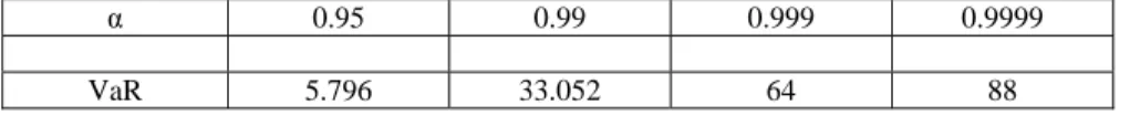
Using result (18.6) we obtain the VaR values given in Table 18.2 according to different security or probability levels.

Į 0.95 0.99 0.999 0.9999

VaR 5.796 33.052 64 88

Table 18.2. VaR values for one asset with the normal distribution

The interpretation of these results uses the frequency interpretation of probability stating that the probability of an event can be seen as the ratio of the “favorable”

cases, i.e. the realization of the considered event, over the total number of realizations, this last one assumed to be large so that this interpretation is confirmed by the law of large numbers.

So, with a level of 0.999, after one year there is one chance in 1,000 that the observed loss is over €64 per action.

If level 0.9999 is imposed, with one chance in 10,000, the loss per action is larger than €88, which is 40% larger than with the preceding level.

For the total of the investment, we obtain the following results.

Į 0.95 0.99 0.999 0.9999

VaR 57,960 330,520 640,000 880,000

Table 18.3. VaR values for the total investment with the normal distribution

In percentage of the global investment, the part of the VaR is given by Table 18.4.

Į 0.95 0.99 0.999 0.9999

VaR 0.00828 0.04722 0.09142 0.1257 Table 18.4. VaR values in percentage of the global investment

with the normal distribution

So, to pass from the minimum level 0.95 up to the maximum level 0.9999, the amount of the VaR is multiplied by 15.18!

Conclusion for example I

This example shows both the interest of the concept of VaR and its difficulties to apply it due to the following:

– the selection a security level D : it is fixed by the supervisor;

– the estimation of the parameters from a good database on historical data of the considered asset and on the considered period;

– the use of normal distribution for the return is called the standard method in Basel I and II and thus there is no problem of authorization for the institution using except the justification of the parameter estimation;

– the risk of obtaining values too high for the VaR. In this case high amounts of equities could not be used for new investments.

18.1.4. Example II: an internal model in case of the lognormal distribution One way for the financial institution to outline the last point is to build its own model, called an internal model, from which a VaR value can be calculated. If this internal model is approved by the supervisor, then the institution can use it instead of the standard method.

As an example, let us start with the assumption that the given asset has a stochastic dynamics governed by the Black and Scholes model seen in Chapter 14 in which we have seen that for such a model for stochastic process (18.1) with trend Pand volatility V , the distribution of S t( ) /S₀ is a lognormal distribution with parameters

2

, 2

2 t t

P V V

§ ·

¨ ¸

© ¹

or

2 2 0

ln ( ) ,

2

S t N t t

S

P V V

§§ · ·

¨¨ ¸ ¸

© ¹

© ¹

E (18.7)

so that:

> @

2

0 2 2 0

( ) ,

var ( ) ( 1).

t

t t

E S t S e S t S e e

P

P V (18.8)

To calculate VaR values at the time horizon T, we have to study the loss given by:

0 0

0

( ) 1 S T( ) ,

S S T S

S

§ ·

¨ ¸

© ¹ (18.9)

and so, we successively obtain:

0 0

0

( ) 1 S T( ) , S S T S

S

§ ·

¨ ¸

© ¹ (18.10)

0 0

0 0

0 0

0 0

1 ( ) ,

1 ( ) ,

1 ( ) ,

ln 1 ln ( ) .

P S S T VaR

S VaR P S T

S S

VaR S T

P S S

VaR S T

P S S

D D

D

D

D D D

D

§ § · ·

d

¨ ¨ ¸ ¸

¨ © ¹ ¸

© ¹

§§ · ·

d

¨¨ ¸ ¸

¨© ¹ ¸

© ¹

§§ · ·

d

¨¨ ¸ ¸

¨© ¹ ¸

© ¹

§ § · ·

d

¨ ¨ ¸ ¸

¨ © ¹ ¸

© ¹

(18.11)

Using the reduced variable, we obtain:

2 2

0 0

ln 1 ln ( )

2 2

.

VaR S T

T T

S S

P T T

D P V P V

V V D

§ § · § · § · ·

¨ ¨ ¸ ¨ ¸ ¨ ¸ ¸

© ¹

© ¹ © ¹

¨ d ¸

¨ ¸

¨ ¸

¨ ¸

© ¹

(18.12)

And so:

2

0

ln 1 2

1

VaR T

S T

D P V

V D

§ § · § · ·

¨ ¨ ¸ ¨ ¸ ¸

© ¹

© ¹

¨ ¸

)¨ ¸

¨ ¸

¨ ¸

© ¹

or

2

0

ln 1 2

1 ,

VaR T

S T

D P V

V D

§ § · § · ·

¨ ¨ ¸ ¨ ¸ ¸

© ¹

© ¹

¨ ¸

)¨ ¸

¨ ¸

¨ ¸

© ¹

(18.13)

from which

2

0

ln 1 2

.

VaR T

S z

T

D

D

P V V

§ · § ·

¨ ¸ ¨ ¸

© ¹

© ¹

To obtain the VaR value, we have to solve the following equation:

2

0

ln 1 2

VaR T

S z

T

D

D

P V V

§ · § ·

¨ ¸ ¨ ¸

© ¹

© ¹

or (18.14)

2

0

ln 1 .

2

VaR z T T

S

D DV P V

§ · § ·

¨ ¸ ¨ ¸

© ¹

© ¹

This last result gives the explicit form of the VaR for the lognormal case:

2

2 0

1

T z T

VaR e S

D V

V P

D

§ ·

¨¨© ¸¸¹

or (18.15)

2

2

0 1 .

T z T

VaR S e

D V

V P

D

§ ·

¨¨© ¸¸¹

§ ·

¨ ¸

¨ ¸

© ¹

Here, we see that the crucial problem in determining this VaR value is to calculate and then to estimate the two basic parameters: the trend and the volatility.

To do this, let us recall the following results (see Chapter 10):

> @

2

0 2 2 0

( ) ,

var ( ) ( 1).

T

T T

E S T S e S T S e e

P

P V (18.16)

By inversion, we obtain the values of the two parametersP V, as a function of the mean and variance of S(T):

> @

0 2

2 2 0

1 ( )

ln ,

1 var ( )

ln(1 ).

T

E S T

T S

S T

T S e ^P

P

V

(18.17)

Let us consider the preceding example for the financial institution having at time 0 10,000 shares, each of value €700 and knowing on the time period T, that the mean return is €60 and the standard deviation 40.

Formula (18.17) gives as a result:

2

0.0822, 0.0027665, 0.052597.

P V V

(18.18)

The second result of (18.15) gives Table 18.5.

alpha 0.95 0.99 0.999 0.9998

VaR 3.95 28.45359 55.232 74.39682

Table 18.5. VaR values for the lognormal distribution

The two next tables compare the results of the two models: standard (normal) and internal (lognormal), first for one asset (Table 18.6) and secondly (Table 18.7) for all the investment.

alpha 0.95 0.99 0.999 0.9999

VaR I 5.796 33.052 64 88

VaR II 3.95 28.45359 55.232 74.39682 Table 18.6. Comparisons of VaR values for one asset between models I and II

For the portfolio, we obtain the following.

alpha 0.95 0.99 0.999 0.9999 VaR I 57,960 330,520 640,000 880,000 VaR II 39,500 284,536 552,320 743,968 Table 18.7. Comparisons of VaR values for the global investment between models I and II

Finally, the VaR values in percentage of the global investment are given by Table 18.8.

alpha 0.95 0.99 0.999 0.9999

VaR I 0.00828 0.04722 0.09142 0.1257 VaR II 0.0056 0.04064 0.07890 0.1062

Table 18.8. Comparisons of VaR values in percentage for the global investment between models I and II

The last table, Table 18.9, gives the VaR I as a percentage of the VaR II.

alpha 0.95 0.99 0.999 0.9999

VaR I 1.479 1.1619 1.1587 1.1836

Table 18.9. VaR I as a percentage of the VaR II

We see that this percentage reduces when the security level D increases.

Conclusion for example II

– Here, the internal model gives lower values than the standard model, and so the institution is lucky to use such a model! It will probably be accepted without any problem as the Black and Scholes model is well used for modeling share evolution.

– These two examples well illustrate the modelization risk as indeed with two acceptable models, we obtain different values of the VaR indicators. This is why the control authorities often use supplementary guarantees; for example, in Basel I, they used the level 0.99 and took a final VaR value three times the value at this level!

– Of course, if the internal model is favorable to the institution this model will be used to calculate VaR values provided this internal model will be validated by the control authorities.

– In any cases, this new VaR value cannot go too low with respect to the standard one, for example a reduction no more than 80%.

18.1.5. Trajectory simulation

When it is not possible to obtain explicit results of the VaR values or even when it is possible it may be useful to simulate N sample paths of the considered asset and observe for each of them the value of the loss at time T, that is, the values

0 _i( ), 1,..., S S T i N

. (18.19)

Then from the histogram of these values, it is possible to deduce an estimation of the VaR at different security levels: VaR_D, Į varying.

Here we must mention that the control authorities always ask the financial institutions to periodically recalculate their VaR values VaR_D.

So, for example, in case of a VaR_D calculated daily for a time period of M days and with the day as time unit, the first simulation called S(1) will give the estimation

( ;1)

VaR M_D valuable for the first day. For the second day, we must perform another simulation staring this time with S(1) S₁(1)

to obtain the estimation of estimation VaR M_D( ; 2), etc. This means that for the j^th day, we will start from

( 1) _i( 1), 2,..., S j S j j M

.

Each sample path (i=1,…,N), will give the observed value ( (S j_i 1) S j_i( ),j 1, 2,...,M1

) from which we deduce the observed VaR values.

18.2. Coherence and VaR extensions 18.2.1. Risk measures

The notion of VaR represents well a risk measure or risk indicator for this investor. Generally, let us consider a given risk represented by the r.v. X, for example the loss at the end of a time period as before, and a risk measure defined as a functional T associated with the given risk a positive T( )X , which provides the level of danger in the economic and financial environment of this investor for the given risk with subjective choice, as before the fixation of the security level D . In practice, T( )X will always be an amount of money representing the capital needed to hedge the given risk, and of course we pose:

(0) 0

T (18.20)

Artzner, Delbaen, Eber and Heath (1999) introduced the concept of coherent risk measure imposing the following conditions:

(i) invariance by translation:T(X c) T( )X c, c;

(ii) sub-additivity: T(X Y)dT( )X T( )Y , for all risks X,Y; (18.21) (iii) homogenity: T(cX) cT( ),X !c 0;

(iv) monotonicity: P X( dY) Ÿ1 T( )X dT( ).Y

With Denuit and Charpentier (2004), the following condition, only useful for insurance, is added:

(v) T( )X tE X( ) (18.22)

stating that the amount of hedging is always higher than or equal to the mean loss.

From property (iii), it follows that if loss X is equal to a constant, then T( )c c, which is a very intuitive condition.

Property (ii) of sub-additivity implies that every diversification leads to a risk reduction or at least does not increase the risk, in conformity with Markowitz’s theory developed in Chapter 17.

Finally, in insurance management, property (v) explains that the ruin event is certain without introducing a load factor in the pure premium of value E(X).

18.2.2. General form of the VaR

In the preceding section we have seen that for a risk measured by the r.v. X having a normal distribution

( _X, 2_X)

XEN m V , (18.23)

the VaR value at level D is given by the quantile of order (1D) (D small!) of the d.f. of X, that is:

X X

VaR_D z_DV m

because (18.24)

X X

^.

P Xdz_DV m D

Now, for a risk X having a general d.f. F_X, the VaR level D satisfies the following equality:

( )

FX VaR_D D (18.25)

and if function F_X is strictly increasing, we obtain:

1( ) .

FX D VaR_D (18.26)

This relation gives the way to calculate the VaR value at a given level provided we know the d.f. of X. The knowledge of this function is in general not easy, and so we can proceed with a parametric model as in the Black and Scholes model in section 1 or use simulation methods.

For such a definition of the VaR, it is possible to show that it defines a risk measure that is invariant under translation, homogenous and monotone but not always sub-additive for every d.f. F_X.

Denuit and Charpentier (2005) give the following counter-example: let X and Y be two independent risks having a Pareto distribution, that is,

1 , 0,

( ) ( )

0, 0.

X Y

F x F x x x

x T E

T

­ § · t

° ¨ ¸

® © ¹

°

¯

(18.27)

but withT E 1 so that:

( ) ( ) , 0.

1 P X x P Y x x x

d d x !

(18.28)

From relation (18.25), we obtain at level D : ( ( )) ( )

1 ( )

VaR X P X VaR X

VaR X

D D

D D

d (18.29)

and so

( ) .

VaR_D X 1D D

(18.30)

From the fact that X and Y have the same distribution, we also obtain:

( ) .

VaR_D Y 1D D

(18.31)

The d.f. of the sum X+Y is given by the following manipulation:

(2)

( ) 0^z ( ) ( ) ( ).

X Y X Y X

F z

³

F zu dF z F z ^(18.32)

A little calculation gives the final result:

2

2 ln(1 )

( ) 1 2 , 0.

2 (2 )

X Y

F z z z

z z

!

(18.33)

If we replace

( ) ( )

z VaR_D X VaR_D Y , (18.34)

we obtain:

( ) ( ) 2 ( ) 2 ,

z VaR_D X VaR_D Y VaR_D X 1D D

(18.35)

and so:

(1 )2 1

(2 ( )) ln .

2 1

FX Y VaR_D X D D D D

§¨© D·¸¹ (18.36)

Now, if the property of sub-additivity was satisfied for this Pareto distribution, we must:

( ) ( ) ( )

VaR_D XY dVaR_D X VaR_D Y (18.37)

and by relation (18.35):

( ( )) (2 ( ))

FX Y VaR_D XY dF VaR_D X (18.38)

or by relations (18.25) and (18.36):

(1 )2 1 2 ln 1

D D

D D D

§ ·

¨© ¸¹ (18.39)

However, this is impossible as the second member of (18.39) is strictly less than .D This contradiction proves well that, in general, VaR is not always a coherent risk measure.

Remark 18.1 Of course, this contradiction does not imply that VaR is never a coherent risk measure whatever the d.f. F_X is, and particularly for the standard case of Basel rules, it is so.

To prove this result, let us consider two risks X and Y such that:

2 2

( , ), ( , ),

( , ) .

X X Y Y

X N m Y N m

X Y

V V

U U

E E

(18.40)

From relation (18.6), we know that:

2 2

( ) ,

( ) ,

( ) 2 .

X X

Y Y

X Y X Y X Y

VaR X z m

VaR Y z m

VaR X Y z m m

D D

D D

D D

V V

V V UV V

(18.41)

As U d1, we obtain:

2 2

( )

2 ( )

X Y X Y X Y X Y X Y

VaR X Y

z m m z m m

D

D V V UV V D V V

d (18.42)

and so from the first two relations of (18.41), we obtain:

( ) ( ) ( )

VaR_D XY dVaR_D X VaR_D Y , (18.43)

thus proving that for the standard case, the VaR is well sub-additive. As an additional result, this result also shows that using the optimal diversification principle of Markowitz, we also reduce the VaR of the optimal portfolio with respect to the sum of all individual VaR of each component.

18.2.3. VaR extensions: TVaR and conditional VaR

The search for new indicators having, if possible, better properties than the VaR begins with the consideration that the fixation of the security level is of course subjective and so, the idea is that we effectively fix this level in a reasonable way at value D but to take into account all the values larger than D, we take the mean of

all the corresponding VaR values to obtain a new indicator called Tail-VaR, denoted ( )

TVaR_D X and defined as:

1 1

( ) ( ) .

TVaR_D X 1 VaR_[ X d

D [

D

³

^(18.44)

With the change of variable [6x, where [ F_X( )x , we obtain:

( )

( ) 1 ( ).

1 ^{VaR X X}

TVaR X xdF x

D

D D

f

³

^(18.45)

It follows that:

( )

( ) 1 ( )

1 VaR X ^X

TVaR X xdF x

D

D D

ª f º

« »

¬

³

¼ ^(18.46)

or:

( ) 0

( ) 1 ( ) ( )

1

VaR X

TVaR_D X E X ^D xdFX x

D

ª º

« »

¬

³

¼ ^(18.47)

and with the same change of variable as above, we obtain:

0

( ) 1 ( ) ( ) .

TVaR_D X 1 E X ^DVaR_D X d[ D

ª º

« »

¬

³

¼ ^(18.48)

As the VaR is a function of D , it is also possible to show that the function TVaR of variable D is also decreasing and so, in particular:

( ) 0( ) ( ).

TVaR_D X tTVaR X E X (18.49)

Of course, from relation (18.44), we also have:

( ) ( ).

TVaR_D X tVaR_D X (18.50)

To continue, let us now consider the loss if this loss is effectively greater than the VaR, that is, what we call a scenario catastrophe. To measure this new risk of catastrophic loss, we introduce three new risk indicators:

(i) the conditional tail expectation or CTE levelD : CTE_D; (ii) the conditional VaR or CVaR at level D : CVaR_D; (iii) the expected shortfall or ES at level D : ES_D.

Their definitions are as follows:

^ `

(i) ( ) [ ( ))],

(ii) ( ) ( ) ( ) ,

(iii) ( ) max ( ), 0 .

CTE X E X X VaR X

CVaR X E X VaR X X VaR X

ES X E X VaR X

D D

D D D

D D

!

ª ¬ ! º¼

ª º

¬ ¼

(18.51)

Clearly, we have:

( ) ( ) ( ).

CTE_D X CVaR_D X VaR_D X (18.52)

Thus, CTE_D(X) represents the expectation value of the total loss given that this loss is larger than VaR_D( )X and CVaR_D(X), the expectation value of the excess of less beyond the VaR_D( )X .

ES_D(X) represents the mean loss leveled at VaR_D( )X .

It is possible to show the following results (Denuit and Charpentier (2004)):

( ) ( ) 1 ( ),

1

( ) ( ) 1 ( ).

1 _X( ( ))

TVaR X VaR X ES X

CTE X VaR X ES X

F VaR X

D D D

D D D

D

D

(18.53)

Moreover, if the d.f. F_X is continuous, we know that in this case ( ( ))

FX VaR_D X D and so the two right members in (18.53) are equal giving the next result

( ) ( ).

CTE_D X TVaR_D X (18.54)

Finally, it is possible to show that the TVaR indicator is coherent.

Example 18.1 The conditional tail expectation CTE_D( )X in the standard case.

For X having a normal distribution of parameters m_X m,V²_X V², let us calculate

( ) ( ( )).

CTE_D X E X X !VaR_D X (18.55)

As:

( ) ( ,

( )

P X y

P X y X x y x

P X x

! ! ! !

! , (18.56)

we have:

( )

( )

( 1 )

( ) ( ( ))

( ( ))

( 1 )

= . 1

X VaR X

X VaR X

E X CTE X E X X VaR X

P X VaR X E X

D

D

D D

D

D

!

!

! !

(18.57)

The value of the denominator is given by

(1 ) _X ,

v

xf dx Q D

f

³

where (18.58)

2 2

( )

2

( ),

( ) 1 .

2

x m X

v VaR X

f x e

D

SV V

With the following change of variable: x m

y V

, we obtain:

2

2 2

2

2

2 2

1

1 2

1 ( ) ,

2

1 1

= ,

2 2

= 1 1 ,

2 .

y X

v v m

y y

v m v m

y

v m

xf dx y m e dy

ye dy m e dy

v m I m

I ye dy

V

V V

V

S V

S V S

V )

S V

f f

f f

f

§ § ·· ¨© ¨© ¸¹¸¹

³ ³

³ ³

³

(18.59)

For the calculation of I₁, we successively have:

2 2

2

2

2 2

-

2 2

2 ,

= ,

. 2

y y

z z

u z

ye dy e d y

e du

e z

f f

f

³ ³

³

^(18.60)

Thus, by the last relation of (18.59):

2 2

( ) 1 2

v m

I e ^V

. (18.61)

Now from the last equality of (18.59), we can write:

2 2

( )

1 2

= 1 ,

2

= ( ) 1 ,

v m X

v

v m

xf dx e m

v m v m

m

V V )

S V

VM )

V V

f §¨© §¨© ·¸¹·¸¹

§¨© §¨© ·¸¹·¸¹

³

where (18.62)

2

1 2

( ) '( ) .

2

x

x x e

M )

S

Returning to relations (18.55), and (18.57), we finally obtain:

( ) ( ( )),

(1 ) ( )

= ,

1

X VaR

CTE X E X X VaR X

VaR xf x dx

D

D D

D D

D

f

!

³

^(18.63)

that is,

( ) ( ) 1 [ ( ) (1 ( ))],

1 ( ) = ( ) .

1

X X

X X

CTE X VaR X z m z

VaR X z m

D D D D

D D

V M )

D V M

D

(18.64)

As the normal distribution is of continuous type, we also have:

( ) ( ).

CTE_D X TVaR_D X (18.65)

Finally, from relations (18.45) and (18.44), we obtain:

( ) (1 )[ ( ) ( )],

( ) ( ) ( ).

ES X TVaR X VaR X

CVaR X TVaR X VaR X

D D D

D D D

D

(18.66)

Remark 18.2

1) With the lognormal assumption, X ELN( ,P V²), Besson and Partrat (2005) show that:

2

2

ln ( )

( ) ( ),

ln ( )

1 .

VaR X

CVaR X e VaR X

VaR X

V D P

D D

D

) P V

V ) P

V

) )

§ ·

¨ ¸

© ¹

§ ·

¨ ¸

© ¹

(18.67)

2) Here, we are directly interested with the loss assumed to be positive without introducing a stochastic dynamic model of the considered asset as in example II.

18.3. VaR of an asset portfolio

As we mentioned in Chapter 17 related to the Markowitz theory, for a portfolio composed of several assets, the main difficulty for applying this theory is the estimation of the variance-covariance matrix of the vector of assets constituting this portfolio.

Of course, this problem also exists when we have to calculate the VaR of such a portfolio of several assets.

Three basic methods can be used to calculate the VaR:

– the method of variance-covariance matrix;

– the simulation method;

– the historic method.

In the next sections, we will briefly describe them.

18.3.1. VaR methodology

Theoretically, it is not difficult to extend the VaR method for one asset to a portfolio composed of n assets.

Let

S t1( ),...,S t_n( ) ,

t

> @

0,T (18.68)

be the stochastic process of the vector of the n considered assets; on [0,T], the relative returns are given by

( ) (0)

, 1,..., (0)

i i

i

i

S T S

i n

[ S

(18.69)

so that:

( ) (0) (0), 1,..., .

i i i i

S T S [S i n (18.70)

If

₁,..., _n

'

x x x

with (18.71)

1

0, 1,..., , 1,

i n

i i

x i n

x t

¦

represents the vector of the percentages of repartition of the considered assets in the global portfolio, we have:

> @

1

( ) ( ), 0,

n i i

S t

¦

x S t t T ^(18.72)

and the return of the given global portfolio

> @

1 1

1

1

( ) (0) ( ) (0),

= ( ) (0) ,

= (0).

n n

i i i i

i i

n

i i i

i n

i i i i

S T S x S T x S

x S T S

x[S

¦ ¦

¦

¦

(18.73)

To continue, we need to introduce the mean vector and the variance covariance matrix of the vector [

[₁,...,[ c_n

:

> @

₁^,..., _n

^,

ij

E m m

[

[

6 V

c

(18.74)

so that for the global portfolio, we obtain from the last equality of (18.73):

> @

> @

1 2

1 1

( ) (0) (0) ,

var ( ) (0) (0) (0) .

m

i i i

i

n n

ij i j i j

i j

m E S T S S x m

S T S S S x x

V V

¦

¦¦

^(18.75)

From these results, it follows that if the vector of returns [ has a multi-normal distribution, then the loss of the global portfolio also has a normal distribution of parameters ^N

^m,V2

^.

Thus, we reach the conclusion that in the standard case, the VaR calculation of the global portfolio of the n assets as similar to the case of the VaR for one asset developed in section 18.1.3, relation (18.6).

In the next section, we will show how to implement this method for real applications.

18.3.2. General methods for VaR calculation 18.3.2.1. The variance-covariance matrix method

This method is also known as the Riskmetrics method developed by J.P. Morgan (1996) under the assumption of the multidimensional normality of the vector of returns.

The three steps of the methods are as follows:

(i) calculate the present value of the portfolio, on the time horizon T;

(ii) estimate the mean return vector and of the variance-covariance matrix that must be actualized every day in principle;

(iii) calculate the VaR at the fixed level D. 18.3.2.2. The simulation method

As always in this case, this method is based on a simulation model for the evolution of the considered assets on the time horizon T, the model depending of course of a number of parameters that must be estimated, and to be useful it needs many simulations.

The steps are as follows:

(i) choose a distribution for the vector of returns on the time horizon T;

(ii) simulate a large number of sample paths on [0,T];

(iii) estimate the VaR at the fixed level D.

18.3.2.3. The historic method (Chase Manhattan Bank 1996)

The basic principle of this method is to assume that the distribution of the asset returns in the future is identical to the one in the past.

Of course, this assumption may only be valid on a relatively short time interval and is very sensitive to the quality of the data.

Its main interest is that no assumption is made on the distribution of the asset returns as we start from the observed data in the past to estimate this distribution.

The main steps are as follows:

(i) calculate the present value of the portfolio, on the time horizon T;

(ii) estimate historical returns on the basis of the retained risk factors (asset values, bond values, exchange rates, options values, etc.);

(iii) calculate the historical values of gains and losses of the considered portfolio;

(iv) estimate the VaR at the fixed level D.

Let us also mention that complementing these three methods, the method of scenarios is often used meaning that we can select stressing scenarios corresponding to catastrophic events, which of course are rare and of very small probability, to see how the VaR and TVaR indicators resist in the extreme situations.

18.3.3. VaR implementation

The use of VaR methods depends on the model retained for the time stochastic evolution of the considered n assets of the portfolio.

From section 18.3.1, using the standard model means that vector ^[

^[₁^,...,[_n

^c

has a multi-normal distribution with mean and variance covariance matrix given by (18.74):

> @

₁^,..., _n

^,

ij

E m m

[

[

6 V

c

(18.76)

so that for the global portfolio, from (18.73), we know that:

> @

> @

1 2

1 1

( ) (0) (0) ,

var ( ) (0) (0) (0) .

m

i i i

i n n

ij i j i j

i j

m E S T S S x m

S T S S S x x

V V

¦

¦¦

^(18.77)

As

0 ( )

S S T m

P z_D D

V

§ d ·

¨ ¸

© ¹

or (18.78)

0 ( )

,

P S S T dz_DVm D

from (18.73), we have for the VaR value at level D : .

VaR_D z_DVm (18.79)

The number of parameters to be estimated for the application of this last result is in general high as indeed, we have the n values of the means, the n values of the variance and the n(n-1)/2 covariance values (for two distinct assets), so that we have n(n+2)/2 parameters.

For example, if n=50, which is not a large number of assets for a big bank, we have 1,300 parameters and for n=100, 5,100 parameters!

In fact, as mentioned in Chapter 17, the situation is the same as for the calculation of the efficient frontier and so the crucial problem is to see how to reduce this high number of parameters to estimate, which is a curse in dimension reducibility.

Two possibilities exist: the first possibility, as in Riskmetrics, is based on the evolution of the financial cash flows producing the returns of the portfolio, and the second on the use of econometric models for the asset market.

18.3.3.1. The Riskmetrics method For the considered portfolio, let

F t_k, _k,k 1,...,m

(18.80)

be the future produced cash flows: at time t_k, the asset will produce a return of value F k_k, 1,..., .m

For the given yield curve, the present value of the portfolio is:

1

(1 ) ^k ,

k

m

t

t k

j

i F

¦

^(18.81)

where

tk

i represents the equivalent annual rate for maturity t_k,k 1,..., .m

It is clear that each cash flow value is random and so must be treated carefully and a complete treatment requires the calculation of the correlations between all the components of the cash flow which, as we have seen above, is a problem with combinatory explosion!

Moreover, there will surely be a lack of enough data.

The proposed solution is called the mapping method in which we redistribute on a restricted number of standard maturities, for example: 1, 3, 6 months, 1, 2, 3, 5, 7,

10, 15, 20 and 30 years, all the maturities of cash flows necessary to analyze the different returns.

This needs to solve the following problem: how to split a cash amount of present value M and maturity t between the two nearest standard maturities retained

1 1

, ( )

k k k k

t t t t and with respective present values M M₁, ₂.

This problem is solved with the introduction of two conditions, the first one imposing the equality of the present values and the second the invariance of the duration (see Chapter 9):

1 2

1 1 2

,

k k .

M M M

tM t M t M

(18.82)

This linear system in M M₁, ₂ has the following unique solution:

1 1 1

2 1

, .

k

k k

k

k k

t t

M M

t t

t t

M M

t t

(18.83)

For variances V V_k², _k²₁,V² of the corresponding returns [ [_k, _k1,[ , we obtain:

2 2 2 2 2

1 1 2 2 12 1 1 2

k k k k

M M M M M

V V V U V V (18.84)

where, of course, U₁₂ is the correlation coefficient between the two cash amounts.

Without any information on it, we use the following two inequalities

^V_k^M₁^V_k1^M₂

^2dV2M2d

^V_k^M₁^V_k1^M₂

² (18.85) If we want retain an assumption of maximum volatility, we have to use the

second inequality and so:

1 1 2

ˆ ^kM ^k M .

M

V V

V (18.86)

This will lead to an overestimation of the VaR and of course the use of the first inequality will lead to a sub-estimation.

These two problems of over and sub-estimation can be avoided using a linear interpolation:

1 2

1 2

(1 ) ,

M ,1 M

M M

V DV D V

D D (18.87)

and the two following conditions:

1 2

2 2 2 2 2

1 1 2 12 1 1 2

,

2 .

k k k k

M M M

M M M M M

V V V U V V

(18.88)

Using the last equality of (18.87) for the substitution of M M₁, ₂, we obtain the following equation for D:

2 2 2 2 2 2

1 1 12 1 12 1 1

( _{k k} 2 _{k k} ) 2 ( _{k k k} ) ( _k ) 0.

D V V V V U D V V U V V V (18.89)

18.3.3.2. VaR for an asset portfolio with Sharpe model

Another way for reducing the number of parameters of the covariance matrix is the use of some economic market models; we will see how this method works with two such models: the Sharpe and the MEDAF models.

Let us consider a market with n assets. If r_j,j 1,...,n represents the return function of asset j, the Sharpe model assumes that the variations of these returns satisfy the following relations:

, 1,...,

j j j j

r I j n

' D E ' H (18.90)

where 'I represents the variation of a reference market on the considered time horizon.

The “slack” variables are assumed to be independent and (0, ²)

j

N V_H . 'I is assumed normal and moreover independent of the slack variables.

As the global variation of the portfolio on the considered period is given by

1

,

n j j j

r n r

'

¦

' ^(18.91)

with

(0), (1) (0)

(0) ,

j j j

j j

j

j

n x S

S S

r S

' (18.92)

we obtain:

> @

1

1 1

,

= .

n

j j j I

j

n n

j j j j I

j j

E r n m

n n m

' D E

D E

ª º

¬ ¼

§ ·

¨ ¸

¨ ¸

© ¹

¦

¦ ¦

(18.93)

Furthermore, we also have:

> @

2

2 2 2

1 1

var .

j

n n

j j I j

j j

r n n _H

' ^§¨ E ^·¸ V V

¨ ¸

©

¦

¹

¦

^(18.94)

Remark 18.3 Fortunately, the independence between the error variables does not imply the independence of the returns of the assets as indeed:

cov(' 'r_i, r_j) E E V_{i j I}2,iz j. (18.95) From this result, it follows that for a portfolio of n assets, the calculation of the n(n-1)/2 covariances reduces to the knowledge of the n beta parameters and the ² volatility of the market index.

Such a calculation seems more realistic and so using the traditional approach of the VaR with the normal distribution, we obtain the following result:

var ( ).

VaR r' z_D 'rE 'r (18.96)

Exercise

Let us consider a portfolio with three assets with n₁ 3,n₂ 6,n₃ 1 satisfying the following Sharpe model:

1 1 1

2 1 1

3 3 3

0.014 0.60 , (0, 0.006),

0.014 0.60 , (0,0.006),

0.200 1.32 , (0,0.012)

r I N

r I N

r I N

H H H H H H

' '

' '

' '

(18.97)

Moreover, the reference market index has a normal distribution N(0.0031,0.0468)

and:

1(0) 120, 2(0) 15, 3(0) 640.

X X X

Calculate the VaR value at confidence level 99%.

Answer: 21.4421.

18.3.3.3. VaR for an asset portfolio with the MEDAF model

Let us consider a portfolio of value S(t) at time t constituted at time 0 with n assets such that in t, x i_i, 1,...,n and S t_i( ) represent successively the number and value of assets of type i 1,...,n.

Thus, we have:

1

( ) ( )

n i i i

S t

¦

x S t ^{. (18.98)}

On time horizon T, we have T:

( ) ( ) (0), ( ) (0)

( ) .

(0)

i i i

i i

i

i

S T S T S S T S

r T S

'

(18.99)

These relations lead to:

1

( ) (0)(1 ( ))

n

i i i

i

S T

¦

x S r T ^{. (18.100)}

The MEDAF model assumes that:

0 0

( ) ( ( ) ) ( )

1,...,

i i m i

r T r r T r T

i n

E H

(18.101)

where

– r_m( )T is the return of the market portfolio S_m on

> @

^{0,T ;}

– r₀ is the non-risky return on the same period;

– r.vs. H_i( ),T i 1,...n are independent, with normal distribution and uncorrelated with the return of the market portfolio so that:

( )_i 0, ( _{i m}) 0, 1,...,

E H E Hr i n; (18.102)

– E_i represents the coefficient Eof i, i=1,…,n.

Using this model, we obtain:

0 0

1 1

( ) (0) ( ( ) ) ( ) ,

(0) ( ) (0)

, ( ) .

(0) (0)

m

n n

i i i i i i

i i

S T S r r T r T

x S T x S

S T S

' E H

E H

E H

ª º

¬ ¼

¦ ¦

^(18.103)

For the mean and variance of the portfolio return, we obtain:

> @

> @

0 0

2 2 2 2

1

( ) (0) ( [ ( )] ) ,

var ( ) ( (0)) ( ) [ (0)] .

(0) m

n i

m i

i

E S T S r E r T r

S T S S

S

' E

' V E V

ª º

¬ ¼

ª º

« »

« »

¬

¦

¼ ^(18.104)

Consequently, the VaR value at confidence level Dis given here by:

var ( ) ( ( )).

VaR_D'r z_D 'S T E 'S T (18.105)

18.3.4. VaR for a bond portfolio

Let us consider a portfolio of value S(t) at time t constituted at time 0 with n bonds such that in t, x i_i, 1,...,n and Q_i( )t represent successively the number and value of bonds of type i 1,...,n.

So, we have:

1

( ) ( )

n i i i

p t

¦

xQ t ^{. (18.106)}

Let X₁,...,X_k be the k risk factors such that:

( ) 1 1( ) ... ( ), 1,..., .

j t a X tj ajkXk t j n

Q (18.107)

The portfolio value at time T is given by:

1

1 1

( ) ( ),

= ( ) ( ).

n j j j

k n

j

j j

p t x t

x a_Q X_Q t Q

¦

Q

¦ ¦

^(18.108)

To simplify, let us work on a time horizon of length 1 on which:

1 1

1 1

1 1

(1) (0),

= [ (1) (0)],

(1) (0)

= (0) ,

(0)

= (0) (0),

(1) (0)

(0) , 1,... .

(0)

k n

j j j

k n

j j j

k n

j j j

p p p

x a X X

X X

x a X

X

x a X r

X X

r k

X

Q Q Q

Q

Q Q

Q Q Q Q

Q Q Q Q

Q Q

Q Q

'

Q

§ ·

¨ ¸

¨ ¸

© ¹

§ · ª º

¨ ¸ « »

¨ ¸ ¬ ¼

© ¹

§ ·

¨ ¸

¨ ¸

© ¹

¦ ¦

¦ ¦

¦ ¦

(18.109)

To calculate VaR values, we must study the k random returnsr_Q(0).

Using for example the historic method, we can obtain the following estimations:

> @

>

_'

@

_'

(0) ˆ ,

cov (0), (0) .

E r m

r r

Q Q

Q Q VQQ (18.110)

Now, from relations (18.109), we