Modeling Intergranular Fracture at Elevated Temperature

Modeling Intergranular Fracture at Elevated Temperature by

Mohd Syahmi Bin Mohd Yusof

Progress report submitted in partial fulfillment of the requirements for the

Bachelor of Engineering (Hons) (Mechanical Engineering)

JUNE 2010

Universiti Teknologi PETRONAS Bandar Seri Iskandar

31750 Tronoh Perak Darul Ridzuan

i

CERTIFICATION OF APPROVAL

Modeling Intergranular Fracture at Elevated Temperaure

by

Mohd Syahmi Bin Mohd Yusof

A project dissertation submitted to the Mechanical Engineering Programme

Universiti Teknologi PETRONAS in partial fulfillment of the requirement for the

BACHELOR OF ENGINEERING (Hons) (MECHANICAL ENGINEERING)

Approved by,

__________________________

(DR. AZMI BIN ABDUL WAHAB)

UNIVERSITI TEKNOLOGI PETRONAS TRONOH, PERAK

JUNE 2010

ii

CERTIFICATION OF ORIGINALITY

This is to certify that I am responsible for the work submitted in this project, that, the original work is my own except as specified in the references and acknowledgements, and that the original work contained herein have not been undertaken or done by unspecified sources or persons.

________________________________

MOHD SYAHMI BIN MOHD YUSOF

iii ABSTRACT

This project presumes modeling intergranular fracture at elevated temperature. The main task is to replicate the journal article by Rishi Raj and M. F. Ashby [1]. The model will be simulated for other materials and applications which relate to intergranular fracture at elevated temperature. By having this model, the time to rupture of material at elevated temperature can be estimated.

There are several types of creep deformation leading to material failure. This project focused only on a type of creep failure which is due to nucleation, growth and coalescence of voids. The work involves two main phases which are replicating the nucleation and growth of voids in single phase materials such as copper and then, expanding the work to more complicated material systems. The model of fixed number of nuclei is done using default data of copper and replicated with other materials containing iron and metal carbides. The model and the results using other metals are shown in the results and discussions section.

Some problems were encountered during modeling of rupture time for continuous nucleation. The results were not as expected when compared to the results presented in the Raj and Ashby’s paper. The main reason is that some of the data used in the paper were not provided. The model for rupture time for fixed number of nuclei and the baseline for the model for continuous nucleation have been successfully created.

iv

ACKNOWLEDGEMENT

First and foremost, the author would like to express his gratitude to Allah S.W.T for give the chance for him to be able to complete the final year project smoothly and successfully within his final year session.

Deepest gratitude to the author’s supervisor, Dr. Azmi Bin Abdul Wahab for his guidance during difficult times, for sharing his experience as a lesson in working life as well as in life and for his support and motivation throughout the two semester supervising the author. Thank you also to Ms Siti Zarinah Binti Mohd Yusof, postgraduate student in technology, for her assistance in completing this project.

Last but not least, the author would like to give special thanks to his family members and colleagues for their support and company in making this final year project a success. Thank you again to all of them.

v

TABLE OF CONTENT

CERTIFICATION . . . . . . . . i

ABSTRACT . . . . . . . . . iv

ACKNOWLEDGEMENT . . . . . . . v

CHAPTER 1 : INTRODUCTION . . . . . 2

1.1 Background of study . . . . 2

1.2 Problem statement . . . . 2

1.3 Objective . . . . . 2

1.4 Scope of study . . . . . 3

CHAPTER 2 : LITERATURE REVIEW . . . . 4

2.1 Creep failures . . . . . 4

2.2 Creep due to void nucleation and growth . 7 2.3 Void geometries . . . . 9

2.4 Intergranular fracture . . . . 12

CHAPTER 3 : METHODOLOGY . . . . . 14

3.1 Flowchart . . . . . 15

3.2 Gantt Chart . . . . . 17

3.3 Modeling time to rupture I . . . 18

3.4 Modeling time to rupture II . . . 20

CHAPTER 4 : RESULTS AND DISCUSSIONS . . . 26

4.1 Time to rupture I . . . . 26

4.2 Time to rupture II . . . . 30

CHAPTER 5 : CONCLUSION . . . . . 35

REFERENCES . . . . . . . . 36

APPENDICES . . . . . . . . 38

vi LIST OF FIGURES

Figure 2.1 Creep curve of strain 4

Figure 2.2 Dislocation configuration of an asymmetrical low-angle

tilt boundary 6

Figure 2.3 Schematic diagram of growth 7

Figure 2.4 Two types of voids which can form at inclusion present in a grain

boundary 8

Figure 2.5 A periodic array of voids in a grain boundary 9

Figure 3.1 Flowchart 15

Figure 3.2 Gantt chart 16

Figure 3.3 Grid graph i versus j for double integration 19

Figure 3.4 Verification result from the coding 24

Figure 4.1 Expected result for fixed number of nuclei 25 Figure 4.2 Time to rupture I (Fixed number of nuclei) 26 Figure 4.3 Graph Comparison between different grain boundary diffusivity

constant, Dbδ of Iron/Iron 27

Figure 4.4 Comparison of metals 28

Figure 4.5 Expected result for continuous voids nucleation and growth 29 Figure 4.6 Continuous nucleation and growth at two grain junction with no

sliding 30

LIST OF TABLES

Table 4.1 Temperature conversion 26

Table 4.2 Diffusivity constant for five iron/iron GB from different references 26 Table 4.3 Diffusivity constant for three different inter 28 Table 4.4 Datasheet for modeling intergranular fracture at elevated

temperature 37

ABBREVIATIONS AND NOMENCLATURES

GB grain boundary

FV a function of energy angles which provides the void volume FS a function of energy angles which provides the void surface area

vii

F_B a function of energy angles which provides the area of the grain boundary which the void occupy

 energy angle formed at the junction of the void and grain boundary DB grain boundary self-diffusion coefficient

δ grain boundary thickness

r radius of curvature of void surface

rB radius of curvature of the projection void in the grain boundary rc critical radius for void nuceation

2l average spacing between the voids

A a fractional measure of the grain boundary area occupied by the voids

 atomic volume

 external applied stress

n local normal stress at the interface which is responsible for void nucleation

 void density of the number of void per unit area in the grain boundary

max maximum number of possible nucleation sites per unit area

c number of critical nuclei per unit area

^ nucleation rate of voids per unit area

pt time dependent probability off adding one vacancy to a nucleus of critical nuclei size

p diameter of the inclusion tr time to fracture in seconds d grain size

1

CHAPTER 1

INTRODUCTION

1.1 Background of study

Application within elevated temperatures normally dealt with creep. Creep is deformation of components which are in service at elevated temperature and exposed to static mechanical stress. At certain condition, creep can be caused by the growth and coalescence of voids on the grain boundaries.

1.2 Problem Statement

Researchers need to have simulation software or model to predict and analyze the failure of materials at the elevated temperature. Thus, it is a need to have a model to estimate the time for materials to fail especially for elevated temperature applications. By producing the model or software, it will help researchers to analyze failures in materials as it can estimate when the materials will fail and this will help in enhancing the respective application. One such application is steam methane reforming, where the reformer tubes are subjected to stresses at high temperature and the main failure mode is creep rupture due to void nucleation and coalescence along the grain boundaries (GB).

1.3 Objective

The objective of this project is to produce a numerical/computational model of intergranular fracture at elevated temperature in which is based on a journal article by Rishi Raj and M. F. Ashby [ 1 ] and the work is divided into two phases:

 Duplicate the model from the journal article;

 Extend the model to simulate other material systems which are related to the elevated temperature application such as steam methane reformer tube.

2 1.4 Scope of study

The modeling of intergranular fracture at elevated temperature will use Microsoft Office Excel as the main tool. As this software is a user friendly and the model or graph in this software easily updated with respect to the formulation and data input.

In Excel, there are a lot of built-in functions and the author could develop a new function in Excel by using the supplied macro language if the function needed is not available.

In this second part of the final year project, the author only keep on with progressing in developing coding in the Visual Basic in Excel as the function of double integration is not provided. The main reference is the journal article “Intergranular Fracture at Elevated Temperature”, by Rishi Raj and M. F. Ashby. [1]

The model is separated into two main tasks which are calculation of the time to rupture for fixed number of nuclei and calculation of rupture time for continuous nucleation. Initially, the author used the GB data for copper as default data in this project. Then, the model will be run using the data from other materials.

3

CHAPTER 2

LITERATURE REVIEW

2.1 Creep Failures

Creep is deformation of components which are in service at elevated temperature and exposed to static mechanical stress, such as the steam methane reformer tubes. Creep is defined as the time-dependent and permanent deformation of materials when subjected to a constant load or stress. Creep is normally an undesirable phenomenon and is often the limiting factor in the lifetime of a part. “According to Material Science and Engineering: An Introduction by William D. Callister”, creep is observed when materials are at temperatures greater than 0.4Tm where Tm is the absolute melting point of the material. [13]

Creep is an important consideration in design in three types of high temperature applications which are:

 the displacement-limited applications in which precise dimensions or mall clearances must be maintained such as in turbine rotors in jet engines;

 rupture-limited applications in which precise dimensions are not essential but fracture must be avoided such as in high pressure steam tubes and pipes;

 stress-relaxation-limited applications in which an initial tension relaxes with time such as in suspended cables and tightened bolts.

In all of these types of applications, design engineers must consider creep deformation and its dependence on time and temperature. Many mechanical systems and components like turbines, steam boilers, and reactors operate at high temperatures and creep properties for the materials used must be determined.

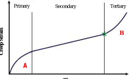
Figure 2.1 Creep curve of strain

Creep fracture is complicated as under creep conditions, fracture most commonly occurs by growth and coalescence of voids which lie on the grain boundaries. The void growth can be controlled by boundary diffusion, surface diffusion, power-law creep, or by coupling of diffusion and power-law creep. This type of fracture depends on the equivalent stress, the magnitude of maximum principal stress and hydrostatic pressure. From the figure about, the graph distributed into three regions as follows [13]:

 Primary creep (Transient) - this region is where the rate of change of strain decreases with time due to strain hardening of material.

 Secondary creep (Steady-state creep) - the strain is increasing linearly with time. From design point of view, this region is the most important for parts designed for long service life because it comprises the longest creep duration.

During this stage, there is a balance between strain hardening due to deformation and softening due to recovery process similar to those occurring in the annealing of metals at elevated temperature.

Creep Strain

Primary Secondary Tertiary

A

A

B

Time

A: Decelerating  strain hardening B: Accelerating  strain softening

5

 Tertiary creep - the strain in this region increases rapidly until failure or rupture. The time to failure normally known as time to rupture, tr. This parameter is an important consideration in designing for parts intended for short-life applications. To determine the rupture time, the creep test must be conducted to the point of failure.

There are several types of creep such as dislocation creep, Nabarro-Herring creep, Coble creep, creep of polymer, Power-Law creep and voids nucleation and growth creep [9] discussed briefly as follows:

 Dislocation creep - This creep is due to the high stresses with relative to the shear modulus which is controlled by the movement of dislocation. The creep has strong dependence on the applied stress and does not dependence on grain size. It takes place due to the movement of dislocation through a crystal lattice. Each time a dislocations moves through a crystal, part of the crystal moves one lattice point along a plane, relative to the rest of the crystal [13].

 Nabarro-Herring creep - The atoms diffuse through the lattice causing grains to elongate along the stress axis. It has weak stress dependence and a moderate grain size dependence, with the creep rate decreasing as the grain size is increased. On the other hand, Nabarro-Herring creep is very dependence towards the temperature. Lattice diffusion of atoms occurs in a material due to the neighboring lattice sites or interstitial sites in the crystal structure are free.

 Coble creep - This creep is a form of diffusion creep which it undergone deformation of crystalline solid and this occur by the diffusion of atoms in a material along the grain boundaries. The diffusion next produces a net flow of material ans a sliding of the grain boundaries. This type of creep is near to the Nabbaro-Herring creep and the difference only at the strain rate and the grain size.

6

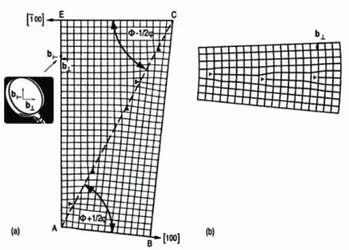
Figure 2.2 Dislocation configuration of an asymmetrical low-angle tilt boundary

 Constant load creep - The rate of constant load creep is a rapidly increasing function of stress. It is usual to distinguish two domains of stress and the first is power-law creep. Power-law creep with a stress component of about 4.5 is quite distinct from creep with the natural law as natural law arise in the solid solutions and having a stress exponent of 3, where the dislocations. It is also rise in pure metals where the rate-controlling process is the annihilation of edge dislocation dipoles by climb.

2.2 Creep due to void nucleation and growth

In ductile failure mechanism, the nucleation, growth and coalescence of voids is a major factor. It is in essence, a result of debonding or cracking at the particles. At first, the high thermal conditions initiate the void nucleation. After a certain period of time, the voids start to grow. The growth will link the voids and finally results in failure of materials. The three sequence process such as void nucleation, void growth and void linkage are in the competition with general plastic localized plastic flow events.

7

Figure 2.3 Schematic diagram of growth

Based on the schematic diagram in Figure 2.2 above, the voids growth in power law creep can be both trans-granular and intergranular, which also influences the void size. The stable nucleated voids grow with respect to time. When the voids reach the critical size, the stress on the remaining area of cross-section will reach the ultimate stress at the temperature and rupture will take place [14].

By referring to J.D Embury, the void nucleation occurs at second phase particles and a variety of criteria. It is also found that, void normally nucleated at the joint of grain boundary. The distances between the nucleated voids are assumed to be the same in order to ease the modeling processes. The nucleation events occur based on local condition where, it may include the local spacing of particles or they are located at the grain boundaries.

For simplicity, two possible extremes for nucleation are the situation where the void nucleation of strain reflects the average volume fraction of particles and decrease slowly with average volume fraction and a condition where nucleation is dominated by the extremes value of particles or inclusion distribution. The void nucleation can be view as a cumulative damage event in which the process de-cohesion spread through the existing particles dispersion. At the high hydrostatic tension the progress of the nucleation may accelerated and the ductility drastically reduced. [11]

8

For void growth, continuum models are being used as it is the problem related to the geometries and the rate of change of the radii of an isolated void in an imposed strain rate field. It is generalized to consider the inter-particles strain. It is clearly state that, the growth dependent on stress state and a table of the relationship between tensile stress, shear stress and mean stress.

2.3 Void geometries

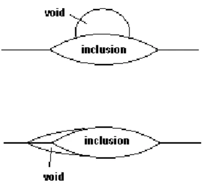
Voids can be differentiated by looking at its geometries as they formed at two-grain, three-grain and four-grain junctions. The same features which the voids have are the free surfaces of the void are spherical segments and the angle between the void must satisfy equilibrium between the surface tension [6].

There two categories of voids. The first category is voids in inclusion-free boundaries and the other is voids at inclusions. The inclusion-free boundaries normally lead to sliding grain boundaries. Besides, there are two types of voids at the inclusion which are Type A, and Type B. For Type A, the void completely lies on the inclusion-matrix interface and Type B is the void extend into the grain boundaries [1].

Figure 2.4 Two types of voids which can form at inclusion present in a grain boundary

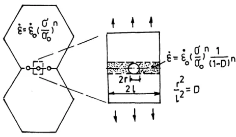
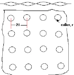
The void growth is estimated in order to know the time-to-fracture of the material. It is assumed that a fixed number of voids exist in an array position and can grow. In reality, there are no fixed numbers of voids as this assumption is made for ease of

calculation. The voids will grow when stress is applied at elevated temperature to the material and the final fracture involves tearing and rapid plastic deformation between the voids.The nucleation of voids must occur before the voids grow and then fail.

Figure 2.5 A periodic array of voids in a grain boundary

The time to rupture for fixed number of nuclei, tr si given by Equation 1 below:

Equation 1

According to above equation, time to rupture for a fixed number of nuclei, tr is the time for the material to rupture as nucleation and growth of voids. The process happens slowly at first and then continues more rapidly.

The term

B D kT

 controls the diffusivity rate for the time to rupture equation. The symbol Ω, represents the atomic volume of material. The atomic volume is defined as the molar mass of an element divided by its density. For the model, the default atomic volume for copper is 1.1 x 10^-29 m³.

    

 





max

2 min 2 3 3

1 32

3 ^A

B A V B

r f A

dA F

F D p

t kT



 



10

Boltzmann’s constant, k with value of 1.380662 × 10⁻²³ J/K is the ratio between the gas constant, R to the Avogadro constant, NA. It is a fundamental constant of physics, occurring in nearly every statistical formulation of both classical and quantum physics. The grain boundary self diffusion coefficient DB for copper is 10^-5exp(- 24.8kcal/mole/RT) m²/sec. It is a measure of particle mobility. The material which have higher self diffusion coefficient implies that the particles can readily diffuse.

The opposite trend happens for the low coefficient [1]. In order to get the accurate result for grain boundary self diffusion coefficient, the Arrhenius equation, exp(- Q/RT) need to be added. R is the gas constant [9]. The boundary thickness, δ for copper is 4x10^-10m.

The

 

³²

1



_p

term determines the external applied load, σ∞ exerted on the void per unit area. The p represents the build up pressure or internal pressure which is assumed to be zero. With a higher density of voids, it would be easier for that certain area to fail as the nucleated voids will grow until it connects with other neighboring voids [1].

The single integration function,

  

max

min A

A f A

dA give the limitation to the possible nucleation site remains. The Amax is the upper limit and Amin is the lower limit.

The geometry of the voids give impact to the time to rupture through the component

32 B

V

F

F where, Fv is a function of angles which provides the void volume and FB is a

function of energy which provides the area B. F_v and F_B will determine the shape of the void. As an example, if the small angle α is inserted into this equation, it will produce a penny-shaped void and if large angle α inserted, it will produce almost a spherical shape. The fractional measures of the grain boundary layer area occupied by voids are represented by A [1].

11

The time to rupture for continuous void nucleation is given by Equation 2:

Equation 2

The value of 0.5 is the limitation for the void density as the material will fail when the right side is more or equal to the left side. The components for this equation act the same as in the time to rupture for fixed number of nuclei. The only difference is the double integration function, ^



^

  

^{ }

 

^

 

^



dtd t

A f t

tr tr



   

0 12

which determines the continuous nucleation for the voids it has the nucleation rate,  _and the possible nucleation site also keep on decrease. This factor leads the equation to become time dependent. The integration is done with respect to the time to rupture.

2.4 Intergranular fracture

Fracture will occur due to the growth of the voids on the grain boundaries. At a certain condition, the void grows by diffusive motion starting with the neighbouring voids. The growth and nucleation of voids within the material have been studied by several metallurgists including Raj and Ashby. There are many aspects that can be used to calculate the time-to-rupture, strain rate, and various interfaces energy.

The time-to-rupture will be calculated in the first place by looking at the void growth and will also apply the nucleation theory to the nucleation-rate of voids. The grain boundaries are separated into two types, one of them is non-sliding boundaries and another one is boundaries which slide. Sliding at the boundaries which appear to have inclusion will lead to the void nucleation as it combines the stress concentration and the high interface energy. The calculation shows that, inclusion is responsible for intergranular fracture [1].

 

               



 







dtd t

A f F t

F kT

D

^{tr tr}

V B

B

   

 

_



0 12 2

/ 3

32

5 3

.

0

12 2.4.1 Elevated temperature failure

The failures at elevated temperature are frequently termed rupture and results from microstructural and metallurgical changes. From this paper it shows that, the main factor for the intergranular fracture to occur is due to the presence of inclusions. The inclusion is typically a distinct particle in the microstructure. It is the place where high stress concentration is exerted and interface energy is also high at this point.

Stress concentration and high interface energy at the inclusion lead to the nucleation of voids [7].

Normally, the growth of void is slow at first and then, it will grow rapidly when local stress rises. For example, the grain boundary separates and forms the internal cracks, cavities and voids. A neck may also form at some point within the deformation region. The elevated temperature condition leads to several effects such as, the instantaneous strain at the time of stress application increases, the steady-state creep rate is increased and the rupture lifetime is diminished.

13

CHAPTER 3

METHODOLOGY

The project, “Modeling Intergranular Fracture at Elevated Temperature” needs further understanding to achieve the objective outlined. The project runs tentatively per flowchart in Figure 6. By referring to the first step, the preliminary research to get the basic understanding about the topic is done.

The project is proceeds by review in depth the Rishi Raj and M.F. Ashby to gain information regarding intergranular fracture at elevated temperatures. Information from journals and books are collected as much as possible for better understanding.

This is to get clear picture about the equations used for every models. After that, by using Microsoft Office Excel to calculate all of the equation and data gathered. The work to replicate this paper by using copper as a default metal data started with modeling the time to rupture with temperature for a fixed number of nuclei in parallel with the time to rupture for continuous nucleation with no grain boundary sliding.

When each of the models done, the model will be tested using other metal data which related to the elevated temperature application.

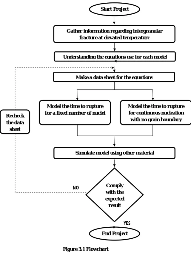
14 3.1 Flowchart

The author starts the project by understanding the journal article. Then, he gathered the basic information regarding intergranular fracture at elevated temperature. He identified which equation from the journal is important to construct the model. There are two main equations for modeling: time to rupture for fixed number of nuclei and time to rupture for continuous nucleation. Next, the data extracted from the journal and arranged in an Excel spreadsheet. The author use Microsoft Excel to do the work.

For the first phase which is to replicate the model, the author starts with the model of time to rupture for fixed number of nuclei. For this model, there is a need for the author to develop a new single integration function using Visual Basic to solve the equation. The integration function done using Simpson’s 1/3 Rule. In parallel, the author also proceeds with time rupture for continuous nucleation model. For this model, the author created a new function of double integration using Simpson’s 1/3 Rule. It is chosen as it is the simplest integration equation. Even though the Simpson’s 1/3 Rule has more error compare to other method, this can be reduced by increasing the number of iterations. The double integration function has been proven to be correct.

When the model is done, the author simulated the model using other materials system. If the result is as per expected, the project can be concluded but, if not, the author need to check the data sheet and the calculation step for the model.

15

Figure 3.1 Flowchart

Simulate model using other material Model the time to rupture

for a fixed number of nuclei

Model the time to rupture for continuous nucleation with no grain boundary Understanding the equations use for each model

End Project Comply with the expected

result

YES NO

Gather information regarding intergranular fracture at elevated temperature

Start Project

Make a data sheet for the equations

Recheck the data sheet

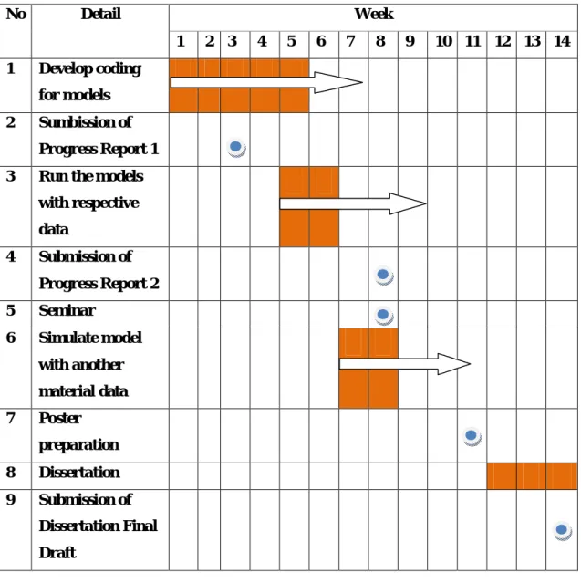
16 3.2 Gantt Chart

Gantt chart below shows the planning for the final year project. The colored region is the expected time to complete certain task. Besides that, there are also arrows which indicated the exact time taken to complete the task.

No Detail Week

1 2 3 4 5 6 7 8 9 10 11 12 13 14 1 Develop coding

for models 2 Sumbission of

Progress Report 1 3 Run the models

with respective data

4 Submission of Progress Report 2 5 Seminar

6 Simulate model with another material data 7 Poster

preparation 8 Dissertation 9 Submission of

Dissertation Final Draft

Figure 3.2 Gantt Chart

17

3.3 Modeling time to rupture I ( Fixed number of nuclei )

In order to solve the equation of time to rupture for fixed number of nuclei, the author needs to treat the equation part by part and at the end compile them together.

The step as per shown below.

3.3.1 Flow to develop the model

The data from the spreadsheet is inserted into equation 2 accordingly and at the end of the equation, there is the integration of area,

  

max

min A

A f A

dA . To solve this, the author used the coding in 3.3.2 below.

3.3.2 Coding

Function inverse_fA(a, rc, r) – to inverse the function of fA/ 1/fA Const e = 2.718281828 – Constant

inverse_fA = a ^ 0.5 * (0.5 * Log(1 / a) / Log(e) - 0.75 + a * (1 - a / 4)) / ((1 - rc / r) * (1 - a))

End Function

Function integrate_inverse_fA(Amax, Amin, n, l, Fb, rc) Const pi = 3.141592654

h = (Amax - Amin) / n

sum_odds = 0 - set the initiation value sum_evens = 0 - set the initiation value A_odds = A_min + h

18 For i = 1 To n - 1 Step 2

r = (pi * A_odds * l ^ 2 / Fb) ^ 0.5

sum_odds = sum_odds + inverse_fA(A_odds, rc, r) A_odds = A_odds + 2 * h

Next i

A_evens = A_min + 2 * h For j = 2 To n - 2 Step 2

r = (pi * A_evens * l ^ 2 / Fb) ^ 0.5

sum_evens = sum_evens + inverse_fA(A_evens, rc, r) A_evens = A_evens + 2 * h

Next j

integrate_inverse_fA = h / 3 * (inverse_fA(Amin, rc, r) + 4 * sum_odds + 2 * sum_evens + inverse_fA(Amax, rc, r))

End Function

Loop to do the iteration for single integration

19

3.4 Modeling time to rupture II (Continuous nucleation, no grain boundary sliding)

Below is the flow in solving the double integration from the Equation 3 in the literature review and the coding. In Excel, the function of double integration is not provided as it is a complex equation which has a lot of different condition in solving the double integration. Due to this, the author needs to code his own coding to come out with the result for the double integration.

3.4.1 Flow to develop the model

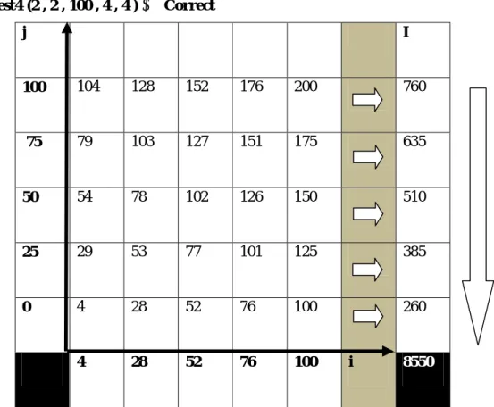
0 1 2 3 4 5 6 7 8 9 tr Figure 3.3 Grid graph i versus j for double integration

From the Figure 3.3, both axes i and j are assumed to start from zero to ten as this is to simplify the calculation afterward. Each point in the grid above represents the value of equation 3 after input the value of i and j. The flow shows as per flow below:

tr 9 8 7 6 5 4 3 2 1 0

j

i

I

I I I I I I I I I

I2

20 i=0 to 10

j=0 to 10 For i=0

J 0 1 2 3 4 5 6 7 8 9 10

Fx F0 F1 F2 F3 F4 F5 F6 F7 F8 F9 F10

For i=1

J 0 1 2 3 4 5 6 7 8 9 10

Fx F0 F1 F2 F3 F4 F5 F6 F7 F8 F9 F10

For i=2

J 0 1 2 3 4 5 6 7 8 9 10

Fx F0 F1 F2 F3 F4 F5 F6 F7 F8 F9 F10

For i=10

J 0 1 2 3 4 5 6 7 8 9 10

Fx F0 F1 F2 F3 F4 F5 F6 F7 F8 F9 F10

Then, when all of the point captured, each row will be inserted into the Simpson’s 1/3 rule for the first integration as per equation 4 below. The same process undergone for each row with respect to the i-axis. The h2 in the equation represents the step size of the equation from one point to another.

3 2 4

2

2

8 , 6 , 4 , 2 1

7 , 5 , 3 , 1

0 n

n

i i n

i

i fx fx

fx fx

h I





















Equation 1 : Simpson’s 1/3 rule (First Integration)

I10

Then, I₀ until I₁₀ put into equation 5 which is the Simpson’s 1/3 rule but with respect to the j-axis. From the second integration, I2 it will give the result of the double integration.

21 3

2 4

1

2

8 , 6 , 4 , 2 1

7 , 5 , 3 , 1 0 2

n n

i i n

i

i Ix Ix

Ix Ix

h I





















Equation 2 : Simpson’s 1/3 rule (Second Integration)

3.4.2 Coding

Public Function DoubleIntegration(rho, rhodot, t, s, n, rc, l, Fb, rb) Dim i As Double

Dim j As Double Dim x As Double Dim y As Double Dim fij As Double Dim rowSize As Double Dim columnSize As Double Dim resultArray() As Double Dim r As Double

Dim Ua As Double Dim NfA As Double Const pi = 3.141592654 Const e = 2.718281828 i = 0

j = s

rowSize = n columnSize = n

ReDim resultArray(rowSize, columnSize) h1 = (t - s) / n

h2 = (t - 0) / n

Ua = ((rb ^ 2) * (j - i)) / (l ^ 2) r = (pi * Ua * l ^ 2 / Fb) ^ 0.5

NfA = ((1 - (rc / r)) * (1 - Ua)) / (Ua ^ 0.5 * (((0.5 * Log(1 / Ua) / Log(e)) - 0.75 + Ua * (1 - (Ua / 4)))))

To set and size the dimensions

Initiation value

Array

Step size of the loop

22 For x = 0 To rowSize

For y = 0 To columnSize

Equation = (rho ^ 0.5) * (j - i) * rhodot * i * NfA resultArray(x, y) = Equation

j = j + h1 Next y i = i + h2 j = s Next x

Dim rowTotal As Double Dim iArray() As Double Dim a As Integer Dim b As Integer

Dim evenTotal As Double Dim oddTotal As Double Dim zeroValue As Double Dim lastValue As Double ReDim iArray(rowSize) rowTotal = 0

For a = 0 To rowSize For b = 0 To columnSize

If (b <> 0 And b <> columnSize) Then If (b Mod 2 = 0) Then

evenTotal = evenTotal + resultArray(a, b) Else

oddTotal = oddTotal + resultArray(a, b) End If

Else

If (b = 0) Then

zeroValue = resultArray(a, b) Else

lastValue = resultArray(a, b) End If

End If

To set and size the dimensions

First integration loop

23 Next b

rowTotal = (h1 / 3) * (zeroValue + (4 * oddTotal) + (2 * evenTotal) + lastValue) iArray(a) = rowTotal

rowTotal = 0 evenTotal = 0 oddTotal = 0 Next a

Dim pointValue As Double Dim z As Integer

Dim iEvenTotal As Double Dim iOddTotal As Double Dim iZeroValue As Double Dim iLastValue As Double For z = 0 To rowSize

If (z <> 0 And z <> rowSize) Then If (z Mod 2 = 0) Then

iEvenTotal = iEvenTotal + iArray(z) Else

iOddTotal = iOddTotal + iArray(z) End If

Else

If (z = 0) Then

iZeroValue = iArray(z) Else

iLastValue = iArray(z) End If

End If

pointValue = (h2 / 3) * (iZeroValue + (4 * iOddTotal) + (2 * iEvenTotal) + iLastValue)

Next z

DoubleIntegration = pointValue End Function

To set and size the dimensions Initiation

Second integration/

Double

integration loop

24

= Test4 (2 , 2 , 100 , 4 , 4 )  Correct

j I

100 104 128 152 176 200 760

75 79 103 127 151 175 635

50 54 78 102 126 150 510

25 29 53 77 101 125 385

0 4 28 52 76 100 260

4 28 52 76 100 i 8550

Figure 3.4 Verification result from the coding

The final value 8550 is proven true by manual calculation. Thus, this show the coding is correct and can be use for the model.

25

CHAPTER 4

RESULTS AND DISCUSSIONS

4.1 Time to rupture I ( Fixed number of nuclei )

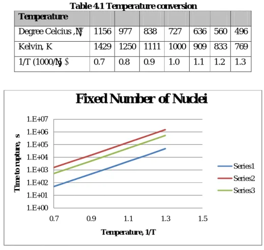
The model for the time to rupture at the fixed number nuclei was simulated using data from other systems operating at elevated temperature. Figure 4.1 shows the expected model for fixed number of nuclei and, Figure 4.2 is the replicated model using the equation of time to rupture for fixed number of nuclei. By referring to Table 4.1, it shows the increment temperature value from 0.7 to 1.3 is actually the decrement of temperature which means, the left side of the graph having higher temperature than on the right side.

Figure 4.1 Expected result for fixed number of nuclei [1]

26

Table 4.1 Temperature conversion Temperature

Degree Celcius ,˚C 1156 977 838 727 636 560 496 Kelvin, K 1429 1250 1111 1000 909 833 769 1/T (1000/˚K) 0.7 0.8 0.9 1.0 1.1 1.2 1.3

Figure 4.2 Time to rupture I (Fixed number of nuclei)

Table 4.2 lists the diffusivity constants, DBδ, for iron/iron GB from various sources.

This is to indicate that there are several diffusivity constants available for certain materials obtained from different references. The legends of Fe/ Fe in the table bring the meaning of grain of iron side with another grain of iron. Figure 4.3 is the result of the different iron constants used in the model of fixed number of nuclei. The slope of each line is almost the same as it is the same material but from different reference.

Table 4.2 Diffusivity constant for five iron/iron GB from different references No Label/ Legend Diffusivity constant, DBδ

1 Fe/Fe 1 5.23E-13

2 Fe/Fe 2 9.18E-11

3 Fe/Fe 3 5.38E-15

4 Fe/Fe 4 2.54E-13

5 Fe/Fe 5 6.79E+13

1.E+00 1.E+01 1.E+02 1.E+03 1.E+04 1.E+05 1.E+06 1.E+07

0.7 0.9 1.1 1.3 1.5

Time to rupture, s

Temperature, 1/T

Fixed Number of Nuclei

Series1 Series2 Series3

27

Figure 4.3 Graph Comparison between different grain boundary diffusivity constant, Dbδ of Iron/Iron

Table 4.3 lists the diffusivity constant, DBδ, for three different interfaces, metals- metal carbide, iron-iron, and copper-copper GB interfaces. The metal-metal carbide, M23C6 is included to the model as metal carbide is usually involved in elevated temperature applications. Figure 4.4, shows the large difference of slope for each metal which is due to the difference in diffusivity constants. The graph shows that Iron-Chromium-Nickel-Carbon-Metal Carbide/ Iron would last longer compared to other materials as the time to rupture of the metal is higher than the other two interfaces.

1.E+02 1.E+03 1.E+04 1.E+05 1.E+06 1.E+07 1.E+08 1.E+09 1.E+10

0.7 0.8 0.9 1.0 1.1 1.2 1.3

Time to fracture (seconds)

1/T (1000/˚K)

Different GB diffusivity constant, D b δ

of Iron/Iron GB

Fe/Fe1 Fe/Fe2 Fe/Fe3 Fe/Fe4 Fe/Fe5

28

Table 4.3 Diffusivity constant for three different inter No Label/ Legend Diffusivity constant, DBδ

1 Iron-Chromium-Nickel- Carbon-Metal Carbide/

Iron

Fe-Cr-Ni-C-M23C6/ Fe

2E-14

2 Iron/ Iron

Fe/ Fe 9.18E-11

3 Copper/ Copper

Cu/ Cu 1.7E-16

Figure 4.4 Comparison of metals 1.00E+02

1.00E+03 1.00E+04 1.00E+05 1.00E+06 1.00E+07 1.00E+08 1.00E+09 1.00E+10

0.7 0.9 1.1 1.3

Time to fracture (seconds)

1/T (1000/˚K)

Graph: Comparison of Metals

Fe/ Fe

Fe-Cr-Ni-C-M23C6 Cu/Cu

29

4.2 Time to rupture II ( Continuous nucleation, no grain boundary sliding )

The result for the time to rupture for continuous void nucleation and growth is not as per expected in Figure 4.5. This is due to the fact that several equations and constants were not provided and the author did not manage to find such as radius of the voids, r at the start of nucleation and the increment of void density,. Due to this, the remaining area at the site could not be estimated. This lead to the nucleation rate,  not functioning properly as it is required as a change in void density, from the results of (_max ) which does not decrease. This is the result from void density being treated as a constant. Supposedly,  is to be treated as a variable due to the fact that void numbers will always increase. When the number of voids increase in a fixed size area, its density proportionally increase. If, keep decreasing, the nucleation rate,  will also decrease. Due to this, the remaining area at the site could not be estimated.

Figure 4.5 Expected result for continuous voids nucleation and growth [1]

30

Even though the model in Figure 4.6 is not as expected, the author already develops the base-line of the models which is the double integration function. The double integration function is successfully done and could function correctly if the radius and the void density increment could be determine and result in the correct curve.

Figure 4.6 Continuous nucleation and growth at two grain junction with no sliding

Below are the steps to solve the models of time to rupture for continuous nucleation, growth and coalescence from the journal by Rishi Raj and M. F. Ashby.

Nucleation and growth of voids: A computer model [1]

A computer model was developed to simulate the continuous nucleation and growth of voids in the grain boundary. Simultaneous nucleation and growth was assumed to occur at a constant rate during small, but discreet, time interval t_ where the subscript determines the sequence of the time intervals. The radius of a void,r_ij, in the jth period depends upon the iith period during which it was born. The number of nuclei of radius,r_ij, _iwill be given by:

i t

i  

 

Equation 3 1.00E+18

1.00E+19 1.00E+20 1.00E+21 1.00E+22 1.00E+23 1.00E+24

0 200 400 600 800 1000

Time to rupture, tr

Temperature, ˚C

Series1

31

Where _iis given by equation (18). When all the nucleation sites, _max, have been exhausted, the nucleation rate goes to zero. New nuclei are assigned the critical radius (equation A 2.13).

Equation 18:











 

 

 



kT F DB kT

n V n

n

2 3 3 max

/ 4

) ( exp 4

) )(

1 4 (





 

 

 

^ 

Equation 4 Equation A2.13:





 2 rc

Equation 5

The computer simulation operates using equations (8 and 2).

Equation 8:







































 























 















 



 



 



 ^

2 2 2

2 2

2

2 2

1 4 4

ln 3

2 1 1

2

l r l

r r

l

l r r l

r kT D dt

dV

B B

B

B B

B B

 

  Equation 6

 sin r

r_B  Equation 7 Equation 2:

)

3 (

V  F r

V  Equation 8



^{ }



  2 3cos cos³ 3

) 2

(   

FV

Equation 9

At every time step, the fraction of grain boundary interface which has been replaced by voids is calculated according to:

)

2 (



_{i ij B}

j r F

A  Equation 10

The value ofj, for whichA_i 0.5, is determined and the time to fracture is then equal to



ⁱ_k₁t_k . If the value j is less than 25, tis increased until j > 25.

Increasing the minimum value of j from 25 to 50 increased the accuracy by only 10

32

percent whereas the computer time needed for the calculation increased logarithmically.

At two-, three- and four-grain junctions, _max was set equal to

2 2

; 2 )) ( (

; 1 )) ( (

1

andd dF

F r

rc B  c B  respectively.

Here d is the grain size, r_c is the radius of a nucleus equal to the volume sum of the critical nucleus plus one atomic volume. _max was taken to be equal to p_p/b² when inclusions were present, pis the inclusion size and _p is the inclusion density in the grain boundary. However, for inclusions, all the nucleation sites were considered to be exhausted when the total number of nuclei was equal to the number of inclusions. The stress in equation (18) was assigned an upper bound value of 2.0X10³MN/m² which was assumed to be the ideal fracture strength of the interface.

All of above steps is from the journal article “Intergranular fracture at elevated temperature” by Rishi Raj and M. F. Ashby. There are several issues with respect to this computer model equation. The value or the equation of radius of the voids,r_ijand the increment of void density, are not provided.

33

CHAPTER 5

CONCLUSION

The modeling of intergranular fracture at elevated temperature by replicating the models from journal, “Intergranular fracture at elevated temperature” by Rishi Raj and M. F. Ashby will help the estimation of the time to rupture for the metals;

especially the ones operating at elevated temperatures as this type of metals are more expensive. Thus, the cost of maintenance and replacements of the components can be controlled.

Creep is the basic principle for the model of time to rupture of voids at the grain boundaries in which creep is the failure mode of materials exposed to elevated temperature for long periods at constant loads or stresses.

The model for time to rupture for the fixed number of nuclei was developed and simulated using data from other GB systems. As shown in Chapter 4, interfaces containing metal carbide, M23C6 last longer at elevated temperatures compared to other materials, as metal carbide is commonly found in metals used for elevated temperature applications. Even though the model of time to rupture for continuous nucleation could not be done due to lack of information, the basis of the model is already completed where the coding for the double integration function uses Simpson’s 1/3 rule.

34

REFERENCES

[1] Rishi Raj and M. F. Ashby (1975). Intergranular fracture at elevated temperature. Acta Metallurgica Vol. 23, 653-666.

[2] R. Raj, H. M. Shih and H. H. Johnson (1977). Correction to: Intergranular fracture at elevated temperature. Scripta Metalurgica, Vol. 11, pp. 839-842.

[3] H.M Tawancy, A. Ul-Hamid, A.I Mohammed and N.M Abbas (2005).

Failure analysis of catalytic steam reformer tube, Emerald Group Publishing Limited.

[4] N. Chandra, P. Dang (1999). Atomistic simulation of grain boundary sliding and migration. Journal of Materials Science 34, 655-666.

[5] David Richards, James B. Adams, and Len Borucki*. Modeling nucleation and growth of voids during electromigration.

[6] Y. Huang and A. Chandra (1998). Void-nucleation vs void-growth controlled plastic flow localization in materials with nonuniform particle distribution. Int. J.

Solids Structures Vol.35, No.19, pp. 2475-2486.

[7] M. Kawai (1998). History-dependent coupled growth of creep damage under variable stress conditions. Metals and Materials, Vol. 4, No. 4, pp. 782-788.

[8] T. Pardoen and J. W. Hutchinson (2000). An extended model for void growth and coalescence. Journal of the Mechanics and Physics of Solid 48, 2467-2512.

[9] F. R. N. Nabarro (2006). Overview No. 141: Creep in commercially pure metals. Acta Metarialia 54, 263-295.

[10] A.C.F. Cocks and M. F. Ashby (1982). On creep fracture by void growth.

Progress in Materials Science, Vol. 27, pp. 189-244.

35

[11] J. D. Embury. Ductile fracture. pp 1089-1103.

[12] B.A Khalifa, M.R.Nagy*, G.S.Al-Ganainy and R.Afify (2006).

Microstructure changes and steady state creep characteristic in the superplastic Sn- 5wt% Bi alloy during transition, Egypt. J. Solids, Vol. 29, No. 1, pp.101-119.

[13] William D. Calister, Jr. (2007) Materials Science and Engineering: An Introduction, Seventh edition. John Wiley and Sons, Inc.

[14] V.M. Radhakrishnan (1986). Rupture life of materials obeying exponential and power law creep, Transactions ISIJ, Vol. 26.

[15] Vincent Gaffard, Jacques Besson, Anne-Francoise Gourgues-Lorenzon (2005). Modeling high temperature creep flow, damage, and fracture behavior of 9Cr1Mo-NbV Steel Weldments, ECCC Creep Conference, pg. 758-768.

[16] Top fired steam methane reformer (SMR). Retrieved August 19,2009, from http://www.kbr.com/technology/Ammonia-and-Fertilizer/Top-Fired-Steam-Methane- Reformer-SMR.aspx

[17] Deformation-mechanism maps: The plasticity and creep of metals and ceramics http://thayer.dartmouth.edu/defmech/

[18] Inderjeet Kaur and Wolfgang Gust (1989): Handbook of grain and interphase boundary diffusion data, volume 2

36 APPENDIX

Raj & Ashby

No. remarks Symbol Data Remarks

1 amu 63.55 atomic mass, g mole^-1

2 density 8.93E+06 atomic density, g m^-3

3 η 6.02E+23 Avogadro's number

4 Ω 1.10E-29 atomic volume, m³

5 k 1.38E-23 Boltzmann's constant, J K^-1

6 R 8.314 gas constant, J mol^-1 K^-1

7 δ 4.00E-10 assumed GB thickness, m

8 not used T 973 absolute temperature, K

9 choose

data

type B

choices: A (estimation) or B (handbook)

10 estimate (D0)est volume diffusion constant, m² s^-1 11 estimate (Q)est volume activation energy, J mol^-1 12 handbook ((DB)0)hb 1.69628E-16 GB diffusivity constant, m³ s^-1 13 handbook (Qb)hb 1.04E+05 GB activation energy, J mol^-1 14 used (δDb)0 1.70E-16 GB diffusivity, m³ s^-1 15 used Qb 1.04E+05 GB activation energy, J mol^-1

16 σ∞ 4.20E+06 applied stress, N m^-2

17 ? γ 0.78 surface free energy, J m^-2

18 from 3D?

void

type A

choices: A (β is active) or B (θ is active)

19 from 3D? β (deg) 1.047197551

void geometry parameters 20 from 3D? θ (deg) 1.047197551

21 Fv 1.308996939

22 Fb 2.35619449

23 Fv/Fb1.5

0.361927787

24 from 3D? ρ 1.00E+10 void density, m^-2

25 from 3D? l 5.00E-06 void-to-void distance, m

26 rc 0.00000001 critical void radius, m

27 Δdt 3600 time step increment

28 Amin 0.0002

29 n 1000

30 h 2.00E-04

31 p 0.00E+00 pressure,Nm^-2

32 ρ^ 0.00E+00 nucleation rate, m^-2s^-1

33 σn 1.0E-04 tensile stress, Nm^-2

34 ρmax 4.24413E+15 maximum void density, m^-2

35 ^ 1.00E-04 strain rate, s^-1

37

36 d 1.00E-05 grain size, m

37 ρp 10000000000 inclusion density, m^-2

38 Ů 0.000000001 imposed sliding rate, ms^-1

39 Dv 1.78396E-26 lattice self-diffusion coefficient, ms^-1

40 p 1.00E-06 diameter of inclusion

41 σ_N normal traction at the interface

Table 4: Datasheet for modeling intergranular fracture at elevated temperature