of the requirements for the Bachelor of

Identification of Source-Receiver Offset for the Presence of Air Wave

by

Mohd Hamka Bin Md Seman

Dissertation submitted in partial fulfillment of the requirements for the

Bachelor of Engineering (Hons) (Electrical and Electronics Engineering)

SEPTEMBER 2011

Universiti Teknologi PETRONAS Bandar Seri Iskandar

31750 Tronoh Perak Darul Ridzuan

CERTIFICATION OF APPROVAL

Identification of Source-Receiver Offset for the presence of Air Wave By

Approved by,

Mohd Hamka Bin Md Seman

A project dissertation submitted to the Electrical and Electronics Engineering Programme

Universiti Teknologi PETRONAS in partial fulfillment of the requirement for the

BACHELOR OF ENGINEERING (Hons) (ELECTRICAL AND ELECTRONICS ENGINEERING)

UNIVERSITI TEKNOLOGI PETRONAS TRONOH, PERAK

September 2011

CERTIFICATION OF ORIGINALITY

This is to certifY that I am responsible for the work submitted in this project, that the original work is my own except as specified in the references and acknowledgements, and that the original work contained herein have not been undertaken or done by unspecified sources or persons.

ABSTRACT

This paper presents the study of new method in finding hydrocarbon reservoirs which is Electromagnetic Sea Bed Logging (SBL ). This study will help to improve the effectiveness of SBL method in shallow water environment. SBL was introduced to overcome some limitations on the recent technology of finding the hydrocarbon reservoirs. Recent technology that is being used widely is seismic method via offset seismic technique which can help to estimate other characteristics of potential hydrocarbon reservoirs such as pore fluid and other rock properties. However, this method cannot distinguish the presence of hydrocarbon reservoir or gas-charged water (saline water) [1]. SBL can curb this problem since it detects the resistivity of the hydrocarbon which is relatively higher than saline water and sediments around it.

However, at shallow water environment, this method will have some limitation due to the presence of the air waves. Air wave is the energy propagates from the source through the atmosphere to the receiver. Since air wave also have high resistivity, thus, it is hard to identify the presence of HC reservoir accurately. The study is started with some literature review first before going to do the simulation. Here, the author presents the literature review that had been done by him and the author also presents together data from Troll West gas Province offshore Norway which uses this method to detect the buried hydrocarbon reservoir. Other than that, the author also presents the methodology time line for his project on this topic.

ACKNOWLEDGEMENT

First and foremost, the author would like to say his appreciation and praise to God for His guidance and blessings throughout the entire course of my Final Year Project. The author also wish to express his gratitude to

Dr.

Afza Bt Shafie, for her supervision and support all the way through completing his Final Year Project as partial accomplishment of the requirement for the Bachelor of Engineering (Hons) of Electrical and Electronics Engineering. The author received an immense amount of guidance, ideas, assistance, support and advice from various figures. Without her help, this Final Year Project may not have been successful. Besides that, the author also would like to credit to Universiti Teknologi PETRONAS, especially to the Electrical and Electronics Engineering Department for giving him the occasion to embark on this project in which has equipped students with essential skills for self-learning. Last but not least, the author would like to thank his lovely family as they have been a wonderful source of encouragement and support to him and not to forget as well his fellow colleagues which gave their effort in ensuring the smooth completion of this project. Their help was a remarkable gift to the author. May God bless all of them, as only HE, the Almighty could recompense them for their benevolence.

TABLE OF CONTENTS

CERTIFICATION OF APPROVAL ii

CERTIFICATION OF ORIGINALITY .

iii

ABSTRACT .

iv

ACKNOWLEDGEMENTS. v

LIST OF FIGURES •

viii

LIST OF TABLES • X

ABBREVIATIONS • xi

CHAPTER I: INTRODUCTION

l

l.l

Background l

1.2

Problem Statement

2

1.3 Objectives

2

1.4

Scope of Study

3

1.5

The Relevancy of the Project . 3

CHAPTER2: LITERATURE REVIEW 4

2.1

Introduction

4

2.2

Seismic Reflection Method.

4

2.3

SBL Method: Principle of Operations.

5

2.4

SBL Method: Operations Methods

6

2.5

SBL: Forward Modelling Result

8

2.6

SBL: Future of the SBL Method

lO

CHAPTER3: METHODOLOGY . 3.1 Project Flow Chart

3.2 Gantt Chart For FYP1 and FYP 2.

3.3 Tools and Equipment Required 3.4 Detailed Procedures

CHAPTER4: RESULTS

AND

DISCUSSION 4.1 Results.

4.2 Discussion

CHAPTERS: CONCLUSION

AND

RECOMMENDATION .

REFERENCES

APPENDICES

12 12 13 15 15

22 22

26

29

30

32

LIST OF FIGURES

Figure 2.1

Interpretation of seismic reflection method after mapping the seafloor.

5

Figure2.2

Simplified geological section Troll West Gas Province.

6

Figure 2.3

Type of signal and the magnitude

7

Figure2.4

The Electric field strength 9

Figure 3.1

Flow chart of the project approach

12

Figure3.2

Gantt Chart for FYP I.

13

Figure3.3

Gantt Chart for FYP 2.

14

Figure3.4

CST Software Icon and Create New Project window.

16

Figure 3.5

Units window .

16

Figure 3.6

Cylinder window

16

Figure3.7

Background Properties

17

Figure3.8

Line window for Tx and

Rx 17

Figure 3.9

Current Path for Tx and Frequency Definition

17

Figure 3.10

Boundary Condition setting window .

17

Figure3.11 LF Frequency Parameters window 18

Figure 3.12 Graph ofE-field from the simulation. 18

Figure 3.13 MATLAB Program Fragment. 20

Figure 3.14 Plotted Graphs from MA TLAB Program 21

Figure4.1 Plotted Graphs from SBL Simulation without HC Presence . 22

Figure 4.2 Plotted Graphs from SBL Simulation with HC Presence 22

LIST OF TABLES

Table 3.1

Parameter used during Simulation

19

Table 4.1

Percentage Difference ofE-field Magnitude .

23

Table 4.2

E-field Magnitude Percentage Difference with HC and without HC.

23

Table 4.3

Value of Source-Receiver Offset at 500m HC Depth Target

24

Table 4.4

Value of Source-Receiver OffSet at 700m HC Depth Target

24

Table 4.5

Value of Source-Receiver Offset at lOOOm HC Depth Target

25

Table 4.6

Value of Source-Receiver Offset without HC Presence 25

Table 4.7

Value of Source-Receiver Offset with HC Presence .

26

LIST OF ABBREVIATIONS

CSEM EM

FYP

HC HED

SBL

Controlled Source Electro Magnetic sounding Electromagnetic wave

Final Year Project Hydrocarbon

Horizontal Electric Dipole

Sea Bed Logging

1.1 BACKGROUND

CHAPTERl INTRODUCTION

Electromagnetic Sea Bed Logging (SBL) is an advanced method developed to detect the presence of hydrocarbon (HC) reservoirs in deep water areas. This method was introduced by the Norwegian oil company, Statoil, commercialized through ElectroMagnetic GeoServices (EMGS) and it is an application of marine Controlled Source Electro Magnetic sounding (CSEM). More than 400 surveys have been run in using this method and several discoveries have been reported [II].

The basic idea of this method is the use of a mobile horizontal electric dipole (HED) transmitter and an array of seafloor electric field receiver. The HED transmitter emits a low frequency of electromagnetic (EM) signal into the water and downwards into the sea bed. The EM signal will be absorbed and travel through the mud and rocks on and under the seabed and then received by the array of receiver. Then, the HC beneath the seafloor is detected when the receiver received signal wave that passed through a very high resistivity medium. This is because HC has the highest resistivity compared to mud and rocks on and under the sea bed.

In addition, the depth of the HC reservoirs also can be measured based on the received signal. This can be known from the value of frequency of the EM signal used. The lower the signal frequency, the deeper the signal can go to detect the HC reservoirs. However, there are several factors that need to be taken into consideration while applying this method in order to ensure the accuracy of the results and data.

Since the transmitter emits the EM wave at every angle, hence the signal propagates everywhere. The receiver then will receive many kind of signal and one of them is air wave signal. This project will discuss the effect of air wave and find the source-receiver offSet where the air waves starts to dominate.

1.2 PROBLEM STATEMENT

OffShore hydrocarbon (HC) exploration is both challenging and expensive. An oil and gas company would loss million dollars if they drill one place and there is no HC reservoir found. Hence, the best HC reservoir detector must be use in order to avoid losses. Seismic exploration is by far the most common tool used to map the buried layer HC reservoir. However, this method will just provide the geological characteristics of the seafloor and the presence of the HC reservoir will be determined by analyzing these characteristics. The presence of HC reservoir is still not 100% can be determined using this data it is not able to define if the potential reservoir is HC or saline water.

The best way to detect the presence of HC reservoir is by using electrical resistivity and Sea Bed Logging (SBL) is a tool that using this method. However, there are still problem will be

faced

for using this method especially at shallow water environment.

The presence of air wave in this environment will make it difficult to identifY the presence of HC reservoir. The air wave will shield the presence of HC reservoir in the seabed. Hence, it's a need to be able to determine the source-receiver offset where the air waves started to dominate.

1.3 OBJECTIVE

• To verifY the presence of air waves in shallow water environment.

• To verifY that air waves shield the presence ofHC reservoir.

• To identifY the range of source-receiver offset where the air waves start to dominate

1.4 SCOPE OF STUDY

The scope of this project consists of research, discussions, and simulation work. The research is important to get ample information regarding on this project. The discussion will be conducted together with the supervisor, project leader and other members that participate in this project in order to keep updated on the progress and information of this project and this will help the author to do this project in efficiently. Then, using CST software, the author will run simulations with the intention of achieving the objectives and get results which later would be analyzed and do improvement on it.

The simulations were done at different seawater depth and different HC reservoir target depth. Then, there will be a program from MATLAB to re-plot data from the simulations and fmd the range where the air waves start to dominate.

1.5 THE RELEVANCY OF THE PROJECT

The aim of this project is to be able to identify the range of source-receiver offset where the air wave started to dominate. Other than that, it is to identify the range of seawater depth where the air waves start to present. After identifying the range, the author will later can exclude that range while analyzing the presence of HC reservoir. This is to make the work of identifying HC reservoir becomes more accurate.

2.1 INTRODUCTION

CHAPTER2

LITERATURE REVIEW

The most important thing in marine geophysics which is being the biggest concern now is to be able to design and develop a technique for the remote which can directly detects the presence ofHC reservoirs underneath the seafloor. Before, people only hoped on the seismic reflection method in order to find HC reservoir but this method is having problem is identifYing the real HC reservoir. Now, the researcher have found a technique that can directly identifY the presence ofHC reservoir using EM wave and this method is called as Electromagnetic Sea Bed Logging (SBL ).

2.2 SEISMIC REFLECTION METHOD

Seismic Reflection method is a widely-used technique using sound waves to image underground rock strata. It is used by earth scientists, and plays an important role in oil exploration. It can be performed on both land and sea [9].

Seismic field acquisition requires placement of acoustic receivers (geophones) on the surface in the case of land exploration, or strings of hydrophones in the water in the case of marine exploration. Seismic data processing is usually done in large computing centers with digital mainframe computers or a large number of processors in parallel configurations.

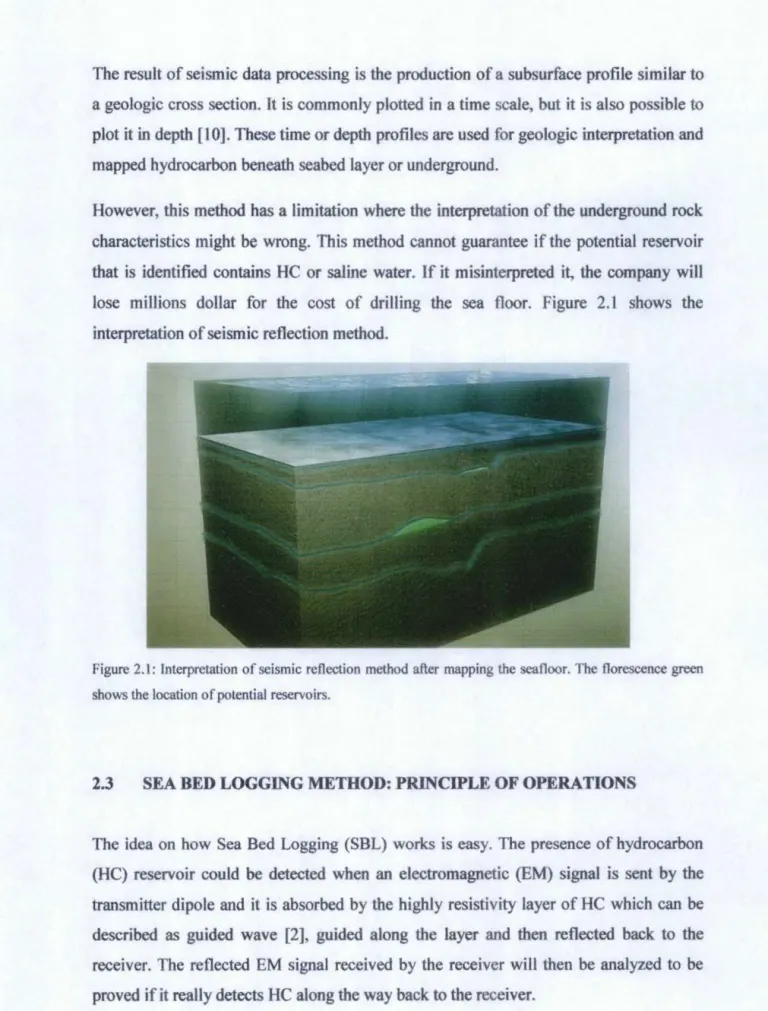
The result of seismic data processing is the production of a subsurface profile similar to a geologic cross section. It is commonly plotted in a time scaJe, but it is also possible to plot it in depth [1 0]. These time or depth profiles are used for geologic interpretation and mapped hydrocarbon beneath seabed layer or underground.

However, this method has a limitation where the interpretation of the underground rock characteristics might be wrong. This method cannot guarantee if the potential reservoir that is identified contains HC or saline water. If it misinterpreted it, the company will lose millions dollar for the cost of drilling the sea floor. Figure 2.1 shows the interpretation of seismic reflection method.

Figure 2.1: Interpretation of seismic reflection method after mapping the seafloor. The florescence green shows the location of potential reservoirs.

2.3 SEA BED LOGGING MEmOD: PRINCIPLE OF OPERATIONS

The idea on how Sea Bed Logging (SBL) works is easy. The presence of hydrocarbon (HC) reservoir could be detected when an electromagnetic (EM) signal is sent by the transmitter dipole and it is absorbed by the highly resistivity layer of HC which can be

described as guided wave [2], guided along the layer and then reflected back to the receiver. The reflected EM signal received by the receiver will then be analyzed to be proved if it really detects HC along the way back to the receiver.

2.4 SEA BED WGGING MEmOD: OPERATIONS MEmODS

The SBL process is done by transmitting EM

signal which is transmitted by a transmitter

which is also known as a horizontal electric dipole (HED) [12]

. This transmitter will

then be towed along the towline and it is towed close to the sea floor. Along the towline, the transmitter will emits a low frequency of EM signal around the dipole and then the reflected signal will be received by the receiver placed on the seafloor.

This

method relies on the large resistivity contrast between HC saturated reservoirs,

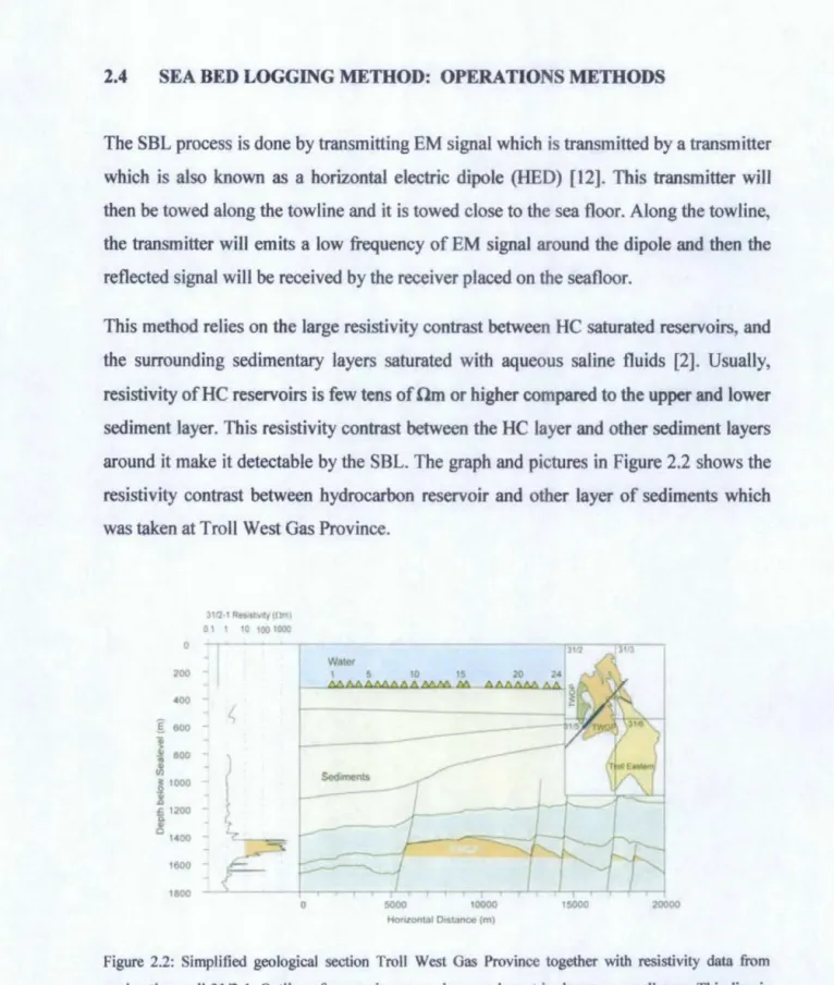
and

the surrounding sedimentary layers saturated with aqueous saline fluids [2]. Usually, resistivity ofHC reservoirs is few tens of Om or higher compared to the upper and lower sediment layer. This resistivity contrast between the HC layer and other sediment layers around it make it detectable by the SBL. The graph and pictures in Figure 2.2 shows the resistivity contrast between hydrocarbon reservoir and other layer of sediments which was taken at Troll West Gas Province.

0

31121ReM!/. !CUm 0 I I 10 tOO 1000

f ^{000 -}

J

^{eoo -}

l j'ooo

ll200

14::10 - 11!00

1800

0 10000 ISOOO 20000

Honzontal Oostance (m)

Figure 2.2: Simplified geological section Troll West Gas Province together with resistivity data from exploration well 3112-l. Outline of reservoir zone and survey layout is shown on small map. Thin line is towline for SBL source and thick line indicates approximate position ofSBL sea floor receiver [6].

However,

the electromagnetic

signal

is emitted

from

all over

the surface of the transmitting dipole which means the

signal

is

not only transmitted towards

the sea

bed

but also towards the sea water surface. In

shallow

water environment, the signal that is transmitted upward to the

sea water surface,

it will get into the air and detect the high resistivity contrast between air and the sea water since the resistivity of

air

is quite high.

This wave is known as 'airwave' and the presents of this wave could bring a problem to the data because the user might interpret the

data as

a detected hydrocarbon

reservoir.

Though, the effect from the airwave

can

be

reduced

by

separation

of total

field

into upgoing and downgoing electromagnetic

wave

fields

[1].

Other than air

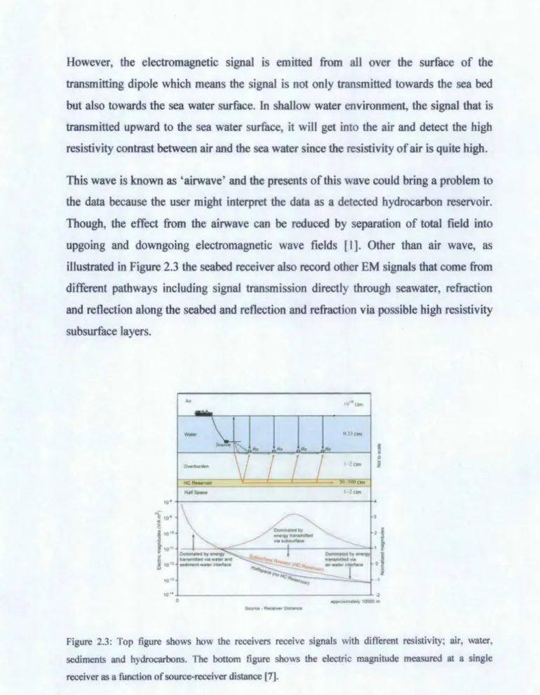
wave,

as illustrated in Figure 2.3 the

seabed

receiver also record other EM signals that come from different pathways including

signal

transmission directly through

seawater, refraction

and reflection along the seabed and reflection and refraction via possible high resistivity

subsurface layers.

1o•,.

10 • ..._ _ _ _ _ _ _ _ _ _ _ _ _ _ __._.:

0 ~IOCICID•

---

Figure 2.3: Top figure shows how the receivers receive signals with different resistivity; air, water, sediments and hydrocarbons. The bottom figure shows the electric magnitude measured at a single receiver as a function of source-receiver distance [7].

The signals that are received by the receiver are:

i. Direct waves from the transmitter

ii. The EM waves reflected back at the boundary of air and seawater (Air waves).

iii. The reflected EM waves from seabed or host rock.

iv. The reflected EM waves from Hydrocarbon.

v. The guided EM waves through Hydrocarbon.

2.5 SEA BED LOGGING: FORWARD MODELING RESULT

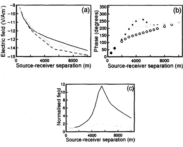
Responses from the horizontal electric dipole (HED) at sea floor can be seen from the graphs in Figure 2.4 below. The graphs demonstrated the effect of thin resistivity layer on the response depends on the source-receiver geometry. There are two geometries that need to be considered:

• In-line geometry - field recorded along a line parallel to the source dipole axis and passing through it.

• Broadside geometry- field recorded along a line perpendicular to the source dipole axis.

The in-line geometry results in a significant contribution to the observed field at the sea floor by the vertical component or current flow. The broadside geometry results in fields at the sea floor that are more dependent on the contribution of inductively coupled currents flowing in horizontal planes. Thus, the presence of the thin resistive reservoir layer produces a significant increase in the in-line geometry, while having low effect on broadside geometry.

The outcome of the signal can be highlighted by normalizing the observed with respect to a reference model. Figure 2.3( c) illustrated the effect of normalizing the signal. The presence of HC layer is not very clear when the source and the receiver are at a short range and at the range of 4-6 km, the amplitude of the in-line response is higher and there is a significant difference between in-line response and broadside response. Thus, in this project, these magnitudes will be considered and recorded for best result and then analyze the relationship between the magnitudes and the result.

~

-9r---,

f=:: '\_, (a)

300~---,

(b)

•

.

. .

•

^{. ... , ..,} 0 u

(ij -12 '

00:: '

o-13 '~:--

·~

'

ti

-14 '

.!! - - -

--- •

w

-15~--._--~--~--_.--~

0 4000 8000

~~--~-4000_. __ _. ___ ^8000._--~

Source-receiver separation (m) Source-receiver separation (m)

12r---~~

~~o

^(c)

1;:::

'08

.~

⁶

"'

E4 ~

0

Z2

0o~--~-4000~--~---8000._--~

Source-receiver separation (m)

Figure 2.4: The electric field strength, the phase of in-line and broadside geometries, and the normalized response as the functions of the source receiver range. The grey line and dots represent the broadside geometry while black line and dots represent in-line geometry.

2.6 SEA BED LOGGING: FUTURE OF THE SBL METHOD

SBL method has been a wide interest in hydrocarbon exploration since a number of success stories on applications of this have been published [8 and 9]. A latest publication [4] evaluates statistical results from wells drilled on prospects or fields containing CSEM data and shows bright future in its application for hydrocarbon exploration.

From 86 wells with associated CSEM data, 36 are calibration surveys collected to test the technology and 50 are exploration wells drilled after the acquisition of CSEM data.

Of the 22 calibration surveys acquired over existing discoveries, 19 (86%) show a significant CSEM anomaly (potential existence of hydrocarbon reservoir). Of the 14 calibration, surveys acquired over prospects that are proven dry, 13 (93%) show no significant CSEM anomaly [5].

When disregarding all calibration surveys, 28 out of 50 wells are discoveries. When considering wells drilled on prospects with a significant CSEM anomaly, 21 out of 30 exploration wells are discoveries. For exploration wells drilled on prospects without a significant CSEM anomaly, 7 out of20 wells are discoveries.

This provides an overall success rate (in terms of technical success regardless of commerciality) of 56%. For wells drilled on prospects with a significant CSEM anomaly, the success rate increases to 70%, whereas it drops to 35% for wells drilled on prospects without a significant CSEM anomaly. As such, the average success rate for wells drilled on prospects with a significant CSEM anomaly is twice the average success rate for wells drilled on prospects without a significant CSEM anomaly.

From exploration point of view, this is important as the technology provides means for the oil companies in finding commercial volumes of hydrocarbons prior to drilling. With the documented success of the technology from empirical data, there should be little doubt about the potential of the technology in the oil industry.

Current challenge in SBL application is it application in shallow water depth. Airwave

components can have severe on the recorded signal and dominate the CSEM response at

source-receiver offsets which are sensitive to structure at the depths of reservoirs. The

key drivers for CSEM data processing and interpretation are estimation and removal of

effects of airwave, seabed topography, shallow carbonates and resistive basement [8].

CHAPTER3 METHODOLOGY

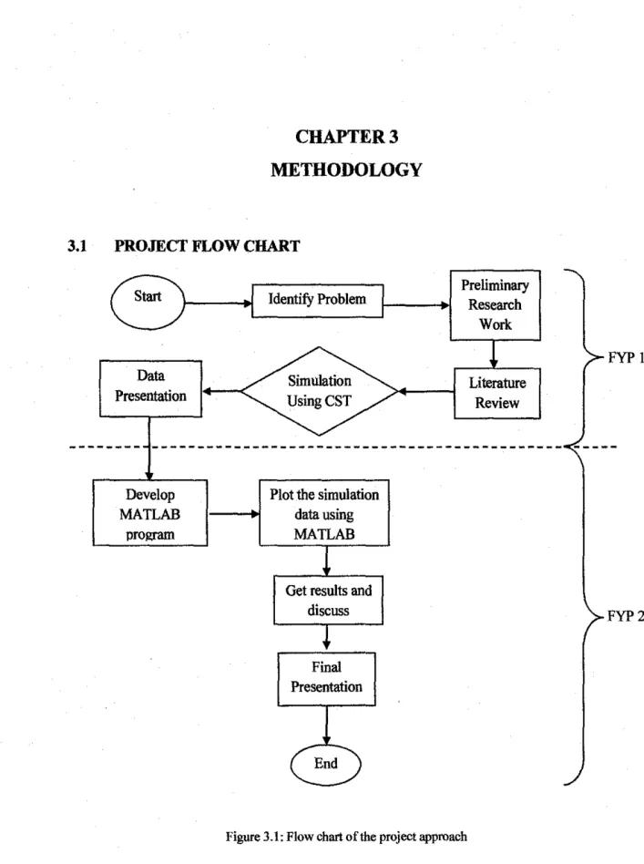
3.1 PROJECT FLOW CHART

Data Presentation

Develop MATLAB

program

IdentifY Problem

Plot the simulation data using MATLAB

Get results and discuss

Final Presentation

Preliminary Research

Work

Literature Review

Figure 3.1: Flow chart of the project approach

FYP I

FYP2

3.2 GANTI CHART FOR FYP 1 AND FYP 2

No 1 2

3

Task Name Selection of Project Topic Preliminary Research Work

Preliminary Report Submission 4 Literature Review

5 Seminar (Proposal Defense and Progress Evaluation) 6 Software Learning

7 Draft Interim Report Submission

8 lnterim Report Submission 9 Oral Presentation

Week

1 2 3 4 5 6 7 8 9 10 11 12 13 14

Figure 3.2: Gantt chart for FYP I

No

1

2

3 4 5

6

7

8

9

Task Name

Project Work Continues Submission of Progress

Report

Project Work Continues Pre-EDX

Week

1 2 3 4 5 6 7 8 9 10 11 12 13 14

Submission of Draft Report

Submission ofDissertation (Soft Bound)

Submission ofTechnical

Paper Oral Presentation Submission of Project Dissertation (Hard Bound)

Figure 3.3: Gantt chart for FYP 2

3.3 TOOLS AND EQUIPMENT REQUIRED

3.3.1 CST Studio Software

This software is for the simulation purposes. It is chosen because this software has the ability to simulate the characteristics of EM wave. This software is also easy to be used which no programming is needed to be done but only design and simulate.

3.3.2 MATLAB software

This software is for the programming part where the author had to do a graph generator programming for data gathered from SBL simulation. This software is chosen because it has a lot of embedded equations and formulas which make the programming process become easier.

3.4 DETAILED PROCEDURES

3.4.1 Identify Problem

At this stage is where the author will identify the problem statement for this project. From here, he and his supervisor can decide the path of this project and the objective for this project. The problems that had been identified are stated in the problem statement.

3.4.2 Research work and data gathering

Research work and data gathering is to help the author to know current status or news that is related to this project. This work also includes the theoretical equations for model development which is done via articles, journals and papers on SBL and EM waves and all these information can be used in the next stage for the development of the seabed logging simulator.

3.4.3 Development ofSBL Simulator

Sea Bed Logging simulator will be done using CST studio software because it bas the electromagnetic simulation and this software is the most efficient and accurate computational solutions to electromagnetic design. Now, the author is still at this stage where be is now in the familiarizing stage.

This is the procedure on how to design the SBL using CST software:

i. Open CST Studio software and create a new project and then choose CST EM STUDIO and then choose "Low Frequency'' for the template.

CST EM STUDIO

~

...

^_,....

- -

Figure 3.4: CST software icon and create new project window

n. Then go to units and then set unit dimension to ''m" and frequency to "hz".

iii. After that, click create cylinder to create the transmitter. Double click on the grid until the cylinder setting window pop out. Then, set the transmitter as shown in the figure beside.

- .__..,

^{. .;;:.} _T- ^laB

•

.

^~

~ r-

IU

. .

.,.,._

Q..-.

-

^~

-

^~

OCJ ^{t.af ~}

Figure 3.5: Units window

- - .. -

^"'

_ ..

^_

- ··

^•

• -

--

^••

_

^•

...

-

^•

-

^•

- ... - ..

-

^I

- , _

- -

^.

...

iv.

v.

vi.

Vll.

Next, start to design the backgrounds which have air, seawater, sediments, and hydrocarbon. Follow the setting in the figure beside.

-:=.:::. __ ..__ __ , , •

-- ....

^.

...

^~

. _ . , _ I

t l I I

~--_no-..~ .._.. .... ,., ...

... .

... "'a ~

... 0.1

--

^{. . . . 4 ...}

._. - - _ - · -

._. .. _ - .. · -

._. -- - _ -·- -

r : ·- .. -·· -.,_.,. -·-.:.J

- . ..

^•

-

^-~

· - ....

^~

...

^,

__ -

.--.,.--,

- - -

^l

Figure 3.7: Background properties

Then, make a curve line for Tx and another for Rx. Follow the setting in the figure beside.

- ..

^'•

"

•

'It

• -

Figure 3.8: Line window for Tx and Rx

After that, make a current

""*c..-,... .._ ,_c-

DofN~,...,

-

F -

.

_~

path at the transmitter, Tx _{a -}^{h 125} _{t..~ J}

1250 ^~

1

and then defme the ^A

...

"'-

frequency. ^{0.0 Deo Oe~ote}

Figure 3.9: Current path window for Tx and frequency definition

Define the boundary conditions to be applied in all directions.

--

_,.,

...

,.. --··· --··· --··· -..:•· -··· -··· •

Figure 3.10: Boundary condition setting window

VIII. Then, define the low frequency domain parameter and simulate the model.

Figure 3.11: LF frequency parameters window

--

.._

_ _

r

ix. Finally, the author should get the result like this. The graph is high at the middle shows the presence of transmitter at that distance and the EM wave reading

is high. _{Figure 3.12:} Graph ofE-field from the simulation

3.4.4 Parameter Variations

CST software is used to simulate the SBL environment for the data used in this research. The main factors considered for the analysis include sea water depth, target depth and source (transmitter}-receiver (Tx-Rx) positions.

The simulations will be based on the following set-up:

i. Fix the source-receiver separation and vary the sea water level to determine the presence of air waves. The purpose of doing this is to get the water level related to the airwaves.

ii. Fix the water level and vary the source-receiver separation distance to determine the presence for air waves. The objective is to get the range of Tx-Rx offset related to presence of air waves.

The sea water level is varied from 1 OOOm to 1OOm at an interval of 1OOm. The source receiver separation is varied from Om to IOOOOm at an interval of 15m. Then, at each level, the Magnitude versus Offset (MVO) plot is done.

The Simulation Parameters:

i. Antenna Length = 150m

ii. Antenna- Sea Bed Distance= 35m iii. Current Used= 1250A

iv. Frequency Used= 0.125Hz

v. Thickness of Hydrocarbon Layer= lOOm vi. Thickness of Over-Burden= 500m vii. Mesh Type =Normal

viii. Range of Sea Water Depth from 1000 -lOOm

Relative Electric Relative

Permittivity (Er) Conductivity (a) Permeability (l'r)

Air 1 0.001 1

Hydrocarbon 4 0.001 I

Sea Water 80 3 I

Sediment 30 1.5 I

Table 3 .I: Parameter used for each elements dunng Slfnulatton

A program in MATLAB will be done to determine the change in the gradient of the curve. This will help to identifY the range ofTx-Rx offset for the presence of airwaves.

3.4.5 Generate Graph from Simulation Data

Simulations had been conducted to get data of Electric field value at different water depth and different source-receiver separation. The simulation is done at two conditions which are one with the presence of HC and another one without the presence of HC. The data obtained from simulation is recorded in tabulated form and then represented in graphical method.

The simulations were done at three different HC reservoir target depth. They were:

i. 500m HC reservoir target depth.

ii. 700m HC reservoir target depth.

iii. 1 OOOm HC reservoir target depth.

Then, a program was developed using MA1LAB to plot graph from the recorded data and find the starting point where the graph started to become steady-state. The program will stop from plotting the graph after finding the point and this is based on the gradient value.

for j=2:668 xG)=DATAG,J);

yG)=DATAQ,2);

mG)=abs((yGl-YG-1))/(xGl-xG-1)));

ifmG)= mG-1)

ifmG-1)<= 0.000000001 break;

else continue;

end else

mG-1);

end i=j-1;

x_axis=DATA(l:i,1);

y_axis= DATA(l:i,2);

end

Figure 3.13: MATLAB program fragment. The program will stop when the gradient's value at certain point is equal to the previous gradient's value and both values are equal to almost zero which is

0.000000001 (9 decimal places)

The plotted graphs are as shown below and the value of x-point where the graph stopped shown in the result part.

Figure 3.14: The graph at the top is the full-plotted graph from the data while another graph is the cut- graph where the graph stops at the point where the gradient value is almost equal to zero.

From the graph plotted, the value of source-receiver offset where theE-field starts to become stable is recorded into tabulated fonn.

4.1 RESULTS

CHAPTER4

RESULTS AND DISCUSSION

The results shown were from the simulations and from the MA TLAB program.

l •

·-

I ;

L .

... -

---- - -

Figure 4.1: Plotted graph from the SBL simuJations without the presence of HC reservoir

l •

I ;

...

I

,

.. - --

-- 1

- --

- -

Sea Water Depth (m) E-field Magnitude Difference (%)

--~-

^6.18

800-900 6.46

~ 6.82

600-700 7.25

!00-600 7.82

400-500 8.71

~ 10.42

200-300 14.22

.... 200 22.77

Table 4. I: E-field magnitude percentage difference at different sea water depth without HC presence

Sea Water Depth 500m HC Depth 700m HC Depth 1000m HC Depth

Target Target Target

1000 ^{63.64 61.96 58.34}

900 62.09 59.28 54.22

800 57.94 54.50 48.16

700 54.03 49.72 41.71

600 50.29 44.88 34.83

500 46.65 39.94 27.48

400 ^{43.15 34.93 19.71}

300 40.00 30.08 11.77

200 37.71 25.97 4.19

100 37.18 23.84 2.18

Table 4.2: Percentage difference of E-field magnjtude between with HC presence and without HC presence at each sea water depth HC depth target

The tabulated data below recorded from the MATLAB programming.

Sea Water

Without HC Reservoir With HC Reservoir Depth(m)

·- 900 3478m 3433m 3378m 3373 m

800 ^{3733m 3403m}

700

^{3403m 3373 m}

600 ^{34S3m 3373m}

500

^{3488m 4018 m}

400 ^{3443m 4048m}

300

^{3373 m 4048m}

180

^{3348m 4SS8m}

100

^{3313 m 4569m}

Table 4.3: Stopped value of source-receiver offset at 500m HC reservoir depth target

Sea Water

Without HC Reservoir With HC Reservoir Depth(m)

·- 900 3478m 3433m 3373m 3388m

800 ^{3733m 3388m}

700

^{3403m 3378m}

600 ^{34S3m 3373m}

500

^{3488m 3403 m}

400 ^{3443m 4048m}

300

^{3373m 3973 m}

180

^{3348m 4118m}

100

^{3313 m 4558m}

Table 4.4: Stopped value of source-receiver offset at 700m HC reservoir depth target

Sea Water

WitboutHC Witb HC

Deptb(m)

1000 ^{3478m 3383m}

900 3433 m 3388m

800 ^{3733m 3388m}

700 3403m 3383 m

600 ^{3453m 3418m}

500 ^{3488m 3388m}

400 ^{3443m 3403m}

300 3373 m 4003 m

100

^{3348m 4048m}

100 3313 m 4018m

Table 4.5: Stopped value of source-receiver offset at l OOOm HC reservoir depth target

Then, the data from the MA TLAB programming were tabulated into 2 categories:

Sea Water SOOm HC Deptb 700m HC Deptb lOOOm HC Deptb

Deptb(m) Target Target Target

1000 ^{3478m 3478m 3478m}

900 ^{3433 m 3433 m 3433m}

800 ^{3733m 3733m 3733m}

700 3403 m 3403 m 3403m

600 ^{3453m 3453m 3453m}

500 ^{3488m 3488m 3488m}

400 ^{3443m 3443m 3443m}

300 3373 m 3373 m 3373 m

100

^{3348m 3348m 3348m}

100 3313 m 3313 m 3313 m

Table 4.6: Stopped value of source-receiver at each depth target without HC presence

Sea Water 500m HC Depth 700m HC Depth lOOOm HC Depth

Depth(m) Target Target Target

·- 900 3378m 3373m 3373m 3388m 3383m 3388m

800 ^{3378m 3388m 3388m}

700 ^{3373 m 3378m 3383 m}

600 ^{3373m 3373m 3418m}

500 ^{4018m 3403 m 3388m}

400 ^{4048m 4048m 3403m}

300 ^{4048m 3973 m 4003m}

200 ^{4SS8m 4118m 4048m}

100 ^{4569m 4558m 4018 m}

Table 4.7: Stopped value of source-receiver at each depth target with HC presence

4.2 DISCUSSION

From Figure 4.1 and Figure 4.2, the difference ofE-field value when the HC reservoir is presence and not presence is obviously shown. The value ofE-field is higher when the HC reservoir is presence like shown in Figure 42. Hence, this is how the HC reservoir is identified.

From Table 4.1, the data was taken from the simulation by CST software without the HC reservoir. It is obvious that the value of E-field increases as the sea water depth is decreases. This situation can be related with the effect of the air wave presence. The presence of air wave is verified since the E-field value is high at 500m sea water depth which can be categorized as shallow water environment. This happened due to the high resistivity value from the air wave presence.

From the tabulated results

at

Table 4.2, the data is the percentage difference of E-field magnitude between with HC presence and without HC presence at each sea water depth and each HC reservoir depth target. From the graph, start from 500m sea water depth and lower, the percentage ditrerence starts to become very low. The very low difference becomes very significant at I OOOm HC reservoir depth target. Since the HC reservoir is deeper, hence the guided wave could not dominate much. Moreover, the presence of air waves also makes the HC presence ahnost undetectable due to very small difference.

From the tabulated results at Table 4.6, the value of source-receiver offset where the E- field value starts to become steady is same for every HC depth target. From the values recorded, at range l000m-600m sea water depth, the trends of the value is not linear.

This is due to the value received at the receiver is not stable and constant.

At range of 500m-l OOm sea water depth, the value is quite linear.

As

the sea water depth decreases, the value of the source-receiver offset where the E-field value starts

to

steady is decreasing as well. This is due to the presence of air wave. As the sea water depth decreases, the air waves reach the receiver earlier at shorter source-receiver offset.

From the tabulated results

at

Table 4.7, the value of source-receiver offset when theE- field value starts to stable is not the same for each HC depth target. At the range I 000m- 600m sea water depth, the recorded offset value is almost the same and the percentage different between each values are not significant.

However, at the range of 500m-1 OOm sea water depth, the percentage different between

the values become larger and more significant. At the 500m HC reservoir depth target, at

500m sea water depth, the recorded offset has large percentage different from the

recorded offset value

at

600m sea water depth. The values then become almost similar

until at 300m sea water depth. At 200m sea water depth, another significant percentage

different happens and it becomes ahnost similar until 1OOm sea water depth. Here, the

presence of air waves starts to dominate at 500 sea water depth environment and it

happens at 4018m source-receiver offset.

For 100m HC reservoir depth target, the significant percentage different of source- receiver offset happened at 400m sea water depth and another one at 1OOm sea water depth. Lastly at 1 OOOm HC reservoir depth target, the significant percentage different happened only at 300m sea water depth. From the data, at 700m HC reservoir depth target, the air wave starts to dominate at 400m sea water depth environment and the domination happens at 4048m source-receiver offset. At I OOOm HC reservoir depth target, the air wave starts to dominate at 300m sea water depth environment and the domination happens at 4003m source-receiver offset.

CHAPTERS

CONCLUSION AND RECOMMENDATION

5.1 CONCLUSION

From the results, a conclusion can be made that the air wave presence starts to become significant at 500m sea water depth and this depth can be categorized as shallow water environment. The presence of air waves really shield the presence of HC reservoir and make the process of identification of HC reservoir become harder. For the source- receiver offset, the air wave starts to dominate at range around 4000m offset.

5.2

RECOMMENDATION

After the source-receiver offset where the air waves start to presence is identified which is around 4000m, further analysis could be conducted by using this information. First, a lab scale experiment must be conducted first to verity the results from the simulation. If the simulation results are correct, future analysis could be done by making this source- receiver offset become fixed and start to quantity the value of the presence air wave.

After the air wave is quantified, then the next survey can just exclude the value contributed by air wave and get more accurate result in identifYing HC reservoir.

REFERENCES

[I] Amundsmen, L., Loseth, L., Mittet,

R.,

Ellingsrud, S. and Ursin, B. [2005]

Decomposition of electromagnetic fields into upgoing and downgoing components. Geophysics, Submitted.

[2] Eidesmo, T., Ellingsrud, S., MacGregor, L.M., Constable, S., Sinha, M.C., Johansen, S.E., Kong, F.N. and Westerdahl, H. [2002] Sea Bed Logging (SBL), a new method for remote and direct identification of hydrocarbon filled layers in deepwater areas, First Break, 20, March, 144-152.

[3] Eidesmo, T., Ellingsrud, S Johansen, S., (2002). Remote sensing of hydrocarbon layers by seabed logging (SBL ): Results from cruise offshore Angola. THE

. LEADING EDGE,

October 2002. 972-982.

[4] Hesthammer, J., Fanavoll, S., Stefatos, A., Danielsen, J.E., & Boulaenko, M., (2010) CSEM performance in light of well results. The Leading Edge.

[5] Hesthammer,

J.,

Stefatos, A., Boulaenko, M., Veresbagin, A., Gelting. P., Wedberg, T., & Maxwell, G., (2010). CSEM technology as a value driver for hydrocarbon exploration. Marine and Petroleum Geology, 27. (1872-1884).

[6] Johansen, S. E., Amundsen, H. E. F., Rosten, Ellingsrud, S., Eidesmo, T., Bhuyian, A. H., (2005). Subsurface Hydrocarbons Detected by Electromagnetic Sounding. First break, 23, 31-36.

[7] Perry A. Fischer., (2005). New EM technology offerings are growing quickly.

WorldOil, Vol. 226, No.6.

[8] Sandeep, K. C., Rashidah Karim.,

Amy

Mawaroi., Russikin Ismail., Noreehan Shahud., Ramlee Rahman., & Paul, B., (2007). Challenges in Shallow Water CSEM Surveying: A Case History from Southest Asia. International Petroleum Technology Conference. (IPTC-11511-PP)

[9] Seismic Reflection Profiling Tutorial. (n.d.). Retrieved March 16, 2010 Retrieved from http://eesc,columbia.edu/courses/ees/lithospherellabs/sonar/sonar.html.

[10] Seismic Exploration for Oil and Gas. (n.d). Retrieved March 15, 2010 Retrieved from http://www.answers.com/topic/seismic-exploration-for-oil-and-gas.

[11] Smit, D., Saleh, S., Voom, J., Costello, M., and Moser, J. [2006] Recent Controlled Source EM results show positive impact on exploration at Shell. SEG Expanded Abstract, Vol25, 2536-3541.

[12] Young, P.D. and Cox, C.S. [1981] Electromagnetic active source sounding near the East pacific Rise. Geophysical Research Letters, 8, 1043-1046.

1.8 X 10·3

1.6

I

e

I

I

^I

~

1 \

<::.

-,:,

u:: a;

g 08

u Cll

w

0.6

0.4

0.2

00 11DJ

E-field Graph for Simulation W1thout HC Presence

200) DXl ^{400) 5(0) 6(0) 71D)} IUD

Source-Receiver Separation (m)

- -11DJm - -!:O:Jm - -EDJm

~ ?oom

--600m 500m - - 400m

- - - - - 3(l)m - - - -2(X)m

--- 100m

!Ull 10CDJ

e; ~

s

('"'}

~ ('J:J

X 10.³

,: ~

I I

161+

I

'

^\ _I

1.4

~

·'I II 1.1 il

E' 1 2 ^{t I} _I

~ , . , ,

II

~ ^I _I

'C 1

'

a; _I

u:: ^I

u ~

u c:

~ 0.8 w

0.6

0.4

I I

I I

Hlll ²⁰⁰⁾

E-1ield Graph for simulation With HC Presence at 500m Depth Target

Dll ^{400) 500) 600)} 700J EDll

Source-Receiver Separation (m)

- -11DJm --900m

- - aoom

·-.. - -700m --GOOm

500m - -400m ---3XIm

---200m ---100m

9(ll)

-

- - - -

-

100J0

2x 10·3

1.8

16 ~

^I

I I

'

^I

14~

e

~

~

"0

'ii u::

u c

~ ^0.8

w 06

0.4

0.2

00 100J ²⁰⁰⁾

E-field Graph for simulation Wrth HC Presence at 100Jm Depth Target

Dll ^{400) 500) 600) 700)}

Sourc&-Receiver Separation (m)

OOll

--100Jm

--900m - -OOJm - - -lOOm

--soom

500m --400m --- DJm

- - - · - 2(X)m --- 100m

9000 ¹⁰⁰⁾⁾