Full Terms & Conditions of access and use can be found at
http://www.tandfonline.com/action/journalInformation?journalCode=ubes20
Download by: [Universitas Maritim Raja Ali Haji] Date: 11 January 2016, At: 22:01
Journal of Business & Economic Statistics
ISSN: 0735-0015 (Print) 1537-2707 (Online) Journal homepage: http://www.tandfonline.com/loi/ubes20
Beyond Stochastic Volatility and Jumps in Returns
and Volatility
Garland Durham & Yang-Ho Park
To cite this article: Garland Durham & Yang-Ho Park (2013) Beyond Stochastic Volatility and Jumps in Returns and Volatility, Journal of Business & Economic Statistics, 31:1, 107-121, DOI: 10.1080/07350015.2013.747800
To link to this article: http://dx.doi.org/10.1080/07350015.2013.747800
Accepted author version posted online: 28 Nov 2012.
Submit your article to this journal
Article views: 426
View related articles
Beyond Stochastic Volatility and Jumps
in Returns and Volatility
Garland D
URHAMLeeds School of Business, University of Colorado, Boulder, CO 80309 ([email protected])
Yang-Ho P
ARKRisk Analysis Section, Federal Reserve Board, Washington, DC 20551 ([email protected])
While a great deal of attention has been focused on stochastic volatility in stock returns, there is strong evidence suggesting that return distributions have time-varying skewness and kurtosis as well. Under the risk-neutral measure, for example, this can be observed from variation across time in the shape of Black– Scholes implied volatility smiles. This article investigates model characteristics that are consistent with variation in the shape of return distributions using a stochastic volatility model with a regime-switching feature to allow for random changes in the parameters governing volatility of volatility, leverage effect, and jump intensity. The analysis consists of two steps. First, the models are estimated using only information from observed returns and option-implied volatility. Standard model assessment tools indicate a strong preference in favor of the proposed models. Since the information from option-implied skewness and kurtosis is not used in fitting the models, it is available for diagnostic purposes. In the second step of the analysis, regressions of option-implied skewness and kurtosis on the filtered state variables (and some controls) suggest that the models have strong explanatory power for these characteristics.
KEY WORDS: Jump intensity; Leverage effect; Option pricing; Regime switching; Return distributions; Skewness; Stock price dynamics.
1. INTRODUCTION
Understanding volatility dynamics and improving option pricing have long been of interest to practitioners and aca-demics. It is well known that the volatility of many financial assets is time varying, and an enormous amount of research has been devoted to studying this feature of financial data. However, there is strong empirical evidence suggesting that return distri-butions have time-varying skewness and kurtosis as well. For example, stochastic skewness in risk-neutral return distributions is implied by variation across time in the slope of the Black– Scholes implied volatility smile. Stochastic kurtosis is related to variation across time in the curvature of the Black–Scholes im-plied volatility smile. These are important features of observed option prices and are only weakly correlated with variation in option-implied volatility. Understanding variation in the shape of return distributions (and the shape of the implied volatility smile) is important in many applications, such as hedging and risk management.
The objective of this article is to investigate model characteris-tics that are consistent with time-varying skewness and kurtosis in return distributions as is observed empirically in the options market. In particular, we look at models with additional state variables that allow for time variation in volatility of volatility, correlation between innovations in prices and volatility (lever-age effect), and jump intensity, all of which are able to generate variation in the shape of return distributions that is independent of the level of volatility. We find strong evidence in favor of these features.
An important aspect of our analysis is that the models are estimated using returns and implied volatility, but additional in-formation about the shape of the return distribution embedded
in option prices (e.g., higher-order moments of the risk-neutral measure) is not used in fitting them. By withholding this infor-mation from the model estiinfor-mation, we are able to use it for diag-nostic purposes. Toward this end, we look at some regressions to examine whether the implied state variables have explanatory power for option-implied skewness and kurtosis and find strong evidence that they do. This is important because it suggests that variation in the shape of risk-neutral return distributions (and of the Black–Scholes implied volatility smile) is not just due, for example, to changes in risk premia, but is associated with changes in related characteristics of the physical dynamics.
This article builds on a substantial body of previous work. Das and Sundaram (1999) showed that both volatility of volatil-ity and correlation between the innovations in an asset’s price and its volatility (leverage effect) affect the shape of the volatil-ity smirk. They showed that the size and intensvolatil-ity of jumps in returns do so as well, although the effect is primarily at short terms to maturities (alternative specifications for the jump dy-namics may be able to generate similar effects at longer hori-zons). There has been some work toward implementing these ideas in empirical work. For example, the two-factor stochastic volatility model of Christoffersen, Heston, and Jacobs (2009) is able to generate time-varying correlation, while Santa-Clara and Yan (2010) allowed the jump intensity to be stochastic. Carr and Wu (2007) proposed a stochastic skew model for foreign exchange rates with positive and negative jumps driven by inde-pendent Levy processes. Johnson (2002) looked at a stochastic
© 2013American Statistical Association Journal of Business & Economic Statistics January 2013, Vol. 31, No. 1 DOI:10.1080/07350015.2013.747800
107
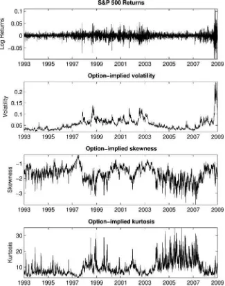
Figure 1. Time series of S&P 500 returns, option-implied volatility, option-implied skewness, and option-implied kurtosis.
volatility model with time-varying correlation between return and volatility innovations. Jones (2003) proposed a constant elasticity of variance model that incorporates a time-varying leverage effect. Harvey and Siddique (1999) looked at gener-alized autoregressive conditional heteroscedasticity (GARCH) models that incorporate time-varying skewness.
The underlying modeling framework is based on a standard single-factor stochastic volatility model. Although models of the affine (or affine-jump) class are often used in work of this kind due to their analytical tractability, these models have trouble
fitting the data (e.g., Jones2003; A¨ıt-Sahalia and Kimmel2007;
Christoffersen, Jacobs, and Mimouni2010). However, since the
techniques applied in this article do not rely upon the analytical tractability of the affine models, we are able to choose among classes of models based on performance instead. We have found that log volatility models provide a useful starting point. We al-low for contemporaneous jumps in both returns and volatility. We build on this framework by adding a regime-switching fea-ture for the parameters corresponding to volatility of volatility, leverage effect, and jump intensity. This idea is motivated by the
fact that changes in any of these three variables, at least under the risk-neutral measure, are capable of generating variation in the shape of the Black–Scholes implied volatility smirk.
Our empirical work uses S&P 500 index (SPX) option data. Figure 1 shows time series plots of option-implied volatility, skewness, and kurtosis estimated using the model-free approach
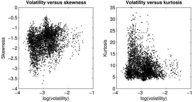
of Bakshi, Kapadia, and Madan (2003).Figure 2shows
scatter-plots of option-implied skewness and kurtosis versus volatility. It is evident from these plots that there is substantial and persis-tent variation in skewness and kurtosis, and that this variation is only weakly correlated with the level of volatility. Models with only a single state variable are hard to reconcile with the em-pirical features of these data. The inclusion of additional state variables in the model (such as the regime states used in this article) is needed to break this lockstep relationship between volatility, skewness, and kurtosis.
The analysis is composed of two main parts. In the first step, we fit the models using SPX prices and option-implied volatil-ity. We compare models based on log-likelihoods, information criteria, and other diagnostics. The second step involves testing
Figure 2. Scatterplots of option-implied skewness and kurtosis against option-implied volatility.
the explanatory power of the implied regime states for option-implied skewness and kurtosis.
Regarding the first step of the analysis, including jumps in the model provides a huge improvement relative to the base model with no jumps. The log-likelihood increases by more than 300 points. Other diagnostics of model fit are also greatly improved. Including the regime-switching feature provides additional large improvements. The best of these models uses regime switching in volatility of volatility. This model provides an increase of 110 points in log-likelihood relative to the model without regime switching, with improvements in other diagnostics of model fit as well.
In the second step of the analysis, regressions testing whether the implied states have explanatory power for option-implied skewness and kurtosis are also decisive. The slope coefficients are strongly significant and in the expected directions. Option-implied skewness tends to be more negative and option-Option-implied kurtosis tends to be more positive when the volatility of volatility is high or the leverage effect is more pronounced (more nega-tive correlation between price and volatility innovations). Our regression results are robust to inclusion of control variables such as VIX index, variance risk premium (VRP), and jump variation. While regression of option-implied skewness on the
control variables alone has an adjustedR2of only 9.2%, adding
the implied regime states to the regression gives an adjustedR2
of over 32%. Slope coefficients for the regime state variables
havetstatistics with absolute value greater than 10.
The remainder of the article is organized as follows: Section
2describes the models under consideration; Section3describes
the methodology; Section4reports parameter estimates and
di-agnostics for the various models; Section5investigates the
ex-planatory power of the implied regime states for option-implied
skewness and kurtosis; and Section6concludes.
2. MODELS
The modeling framework used in this article is based on a standard stochastic volatility model. In light of findings by, for example, Eraker, Johannes, and Polson (2003), we allow for jumps in both returns and volatility. Given a probability space
(,F,P) and information filtration{Ft}, the ex-dividend log
stock price,yt, is assumed to evolve as
dyt =
µ−µ1J tλ1(st)− 1
2exp(vt)
dt
+exp(vt/2)dW1t+J1tdN1t,
dvt =[κ(v−vt)−µ2J tλ1(st)]dt+σ(st)dW2t+J2tdN1t,
dst =(1−2st)dN2t, (1)
wherevt andstare the volatility state and the regime state,
re-spectively. The regime state is either 0 or 1. HereW1tandW2t
are standard Brownian motions with regime-dependent
corre-lationρ(st);N1t andN2t are Poisson processes with intensity
λ1(st) andλ2(st), respectively.
We consider two different forms for the jump structure, depending upon whether jumps are scaled by the volatility state or not. The unscaled models (UJ) assume that jump
innovations are iid bivariate normal with J1t∼N(µ1J, σ12J),
J2t ∼N(µ2J, σ22J), and corr(J1t, J2t)=ρJ. Similar jump
spec-ifications have been used in the existing literature (e.g., Eraker,
Johannes, and Polson2003; Eraker2004; Broadie, Chernov, and
Johannes2007). In contrast, the scaled models (SJ) assume that
jumps scale in proportion to the volatility of the diffusive
com-ponent of the process. That is,J1t andJ2t are bivariate normal
with J1t/exp(vt/2)∼N(µ1J, σ12J), J2t/σ(st)∼N(µ2J, σ22J),
and corr(J1t, J2t)=ρJ. By generating larger jumps when
volatility is higher, the SJ model is potentially capable of provid-ing more realistic dynamics (this hypothesis is indeed confirmed in the empirical section). In either case, we denote the expected jump size (conditional on the volatility state for the SJ models)
byµ1J t =E(eJ1t −1) andµ2J t =E(J2t).
The regime-dependent parameters,σ, ρ, andλ1, allow for
variation across time in the volatility of volatility, leverage ef-fect, and jump intensity, respectively. These are the mechanisms by which it is possible to generate time-varying skewness and
kurtosis. The regime dependence ofλ2lets the regimes differ in
persistence.
For simplicity, we only look at models with two possible regimes, although extending our techniques to more regimes is
straightforward (at the cost of more free parameters to estimate). The regime state process is the continuous-time analog of a discrete-time Markov switching model in which the probability
of switching from statesto state 1−sisλ2(s)t(s=0,1).
While the dynamics of the underlying asset are described by the above model, options are priced according to a risk-neutral
measure,Q. We assume that under this measure, the model takes
the form
wherert andqt denote the risk-free rate and the dividend rate,
respectively; W1Qt and W2Qt are standard Brownian motions
with regime-dependent correlationρ(st) under the risk-neutral
measure.
Jump parameters are the same under physical and risk-neutral measures. In other words, we do not attempt to identify any jump risk premia. The models and data used in this article have limited power to separately identify jump risk and diffusive volatility premia, and our results do not depend on being able to do so.
In empirical work, the VRP is generally found to be negative
(e.g., Coval and Shumway2001; Bakshi and Kapadia2003; Carr
and Wu2009). This finding can be understood in the framework
of classic capital asset pricing theory (e.g., Heston1993; Bakshi
and Kapadia2003; Bollerslev, Gibson, and Zhou2011), but this
theory also suggests that the VRP should be dependent on both the volatility of volatility and the leverage effect (correlation between returns and changes in the volatility state). We allow for this possibility by letting the volatility risk premium parameter
η(st) be regime dependent.
The application looks at several variants of this model,
sum-marized inTable 1. We also looked at a number of alternative
specifications with different regime states, jump dynamics, and risk premia, but do not report results for such experiments to keep the presentation manageable.
In the empirical work, we use an Euler scheme approximation to the model. For the physical model (and analogously for the
Table 1. Summary of models
SV No jumps, no regime switching
SJ Volatility-scaled jumps, no regime switching UJ Volatility-unscaled jumps, no regime switching SJ-RS-Vol Volatility-scaled jumps, regime switching forσ
UJ-RS-Vol Volatility-unscaled jumps, regime switching forσ
SJ-RS-Lev Volatility-scaled jumps, regime switching forρ
UJ-RS-Lev Volatility-unscaled jumps, regime switching forρ
SJ-RS-Jmp Volatility-scaled jumps, regime switching forλ1 UJ-RS-Jmp Volatility-unscaled jumps, regime switching forλ1
risk-neutral model), the approximation is given by
yt+1 =yt+µ−µ1J tλ1(st)−
in the continuous-time model. The regime state,st, follows the
discrete-time Markov process with p(st+1=i|st =j)=Pij,
corresponding to the transition matrix
P=
For computational purposes, we impose an upper-bound con-straint of five jumps in a single day.
3. METHODOLOGY
The introduction of the regime-switching feature means that the models used in this article require the development of new estimation techniques. While the estimation strategies used in similar work often rely heavily on computationally costly sim-ulation methods, the approach we propose in this article runs in several minutes on a typical desktop PC. Our approach con-sists of three steps: (a) back out volatility states from observed option prices; (b) filter regime states using a Bayesian recur-sive filter; and (c) optimize the likelihood function using the volatility and regime states obtained in the previous two steps. As by-products, the algorithm provides a series of generalized residuals, which we make use of for model diagnostics, and estimates of the volatility and regime states, which are used for
the regressions in Section5. A detailed description of each step
of the procedure is provided next.
3.1 Extracting the Volatility States
Building on the work of Chernov and Ghysels (2000), Pan (2002), A¨ıt-Sahalia and Kimmel (2007), and others, we make use of observed option prices in addition to the price of the underlying asset to estimate the models. Estimates of option-implied volatility are obtained using the model-free approach of Bakshi, Kapadia, and Madan (2003).
We now describe the mechanics of how volatility and regime states are backed out conditional on an observed value of option-implied volatility (together with a candidate model and param-eter vector). Following Bakshi, Kapadia, and Madan (2003), let
IVT
t denote the square root of the expected integrated variance
of log returns on the interval (t, T] under the risk-neutral
mea-sure. Given a risk-neutral model for stock price dynamics and initial values for the volatility and regime states, the
correspond-ing value for IVTt can be obtained by integrating the quadratic
variation of the log stock price. For the SJ models (including any of the regime-switching variants), for example, we get
IVTt =
The integrand is equal to the instantaneous variance, which is composed of terms reflecting the diffusion and jump compo-nents of returns. The expectation in the above expression can be computed by means of Monte Carlo simulations,
IVTt ≈
ing paths from the risk-neutral analog of Equation (3) for t < τ ≤T, andSdenotes the number of simulation paths. The calculations for the UJ models are similar, except the integrand
is evτ +λ
1τ(µ21J+σ
2
1J), reflecting the fact that the diffusive
component of returns is scaled by volatility, but not the jumps. However, we actually want to go in the reverse direction.
That is, observed values for IVT
t are available and we need to
obtain the corresponding volatility and regime states,vt andst,
by inverting Equation (4). We begin by showing how to do this conditional on the regime state (the issue of backing out the regime state is addressed in Section 3.2).
Given an initial value for the regime state,st =i, the first
step is to obtain an approximation to the mapping from spot to integrated volatility,
Ŵi: SV−→IV,
where SV denotes the spot volatility, that is, SVt =exp(vt/2),
and the subscript idenotes the conditioning on initial regime
state. The simplest way to do this is to evaluate (4) on some grid of initial values for SV and then use some curve-fitting
tech-nique to approximateŴi. That is, letSV1<SV2<· · ·<SVG
be the grid, whereGis the number of grid points and we use
hats to indicate that these are grid points rather than data. For eachg=1, . . . , G, evaluateIVg =Ŵi(SVg) using Monte Carlo methods as described above (note that while the initial regime state is given, it evolves randomly thereafter). Then
approxi-mateŴi based on the collection of pairs{(SVg,IVg)}Gg=1. As
long as this mapping is monotonic, it is equally straightforward
to approximate the inverse,Ŵ−i1: IV−→SV, which is what
we are really interested in. LetŴi−1denote the approximation.
While there are many curve-fitting schemes one could use, we have found that simply fitting a cubic polynomial to the
collec-tion{(IVg,SVg)}Gg=1using nonlinear least squares works well.
We useG=15 for the empirical work reported in Sections4
and5. We also tried more grid points, higher-order polynomi-als, splines, and various other interpolation schemes, but none provided notable improvements. Approximation errors are neg-ligible for any reasonable scheme.
Given an observed value for option-implied integrated
volatil-ity, IVt, and assumingst =i, one evaluatesŴi−1to obtain SVt.
Then, the volatility state itself is given byvt =2 log(SVt). The
important thing to note here is that computingŴi−1, which is the
costly step, need only be done once (for each candidate
param-eter vector). Once this is accomplished, the evaluation step is fast.
3.2 Filtering the Regime States
Given an observed value of IVt, we now have two possible
values for SVt(andvt), one for each regime state. Letv
j
t denote
the volatility state corresponding to regimej. The second step
of the estimation involves applying a filter to compute ptj =
p(st=j|Ft)=p(vt =v j t|Ft).
The filter is constructed recursively using standard
tech-niques. Letpt=(pt0, pt1)′for eacht =0, . . . , n, and initialize
the filter by settingpj0equal to the marginal probability of state
j(j =0,1). Now, suppose thatptis known. The problem is to
The third factor in the summand is known from the previous step of the recursion. The second factor is determined by the Markov transition matrix of the regime state process. For the first factor, since we allow for the possibility of more than a single jump per day, it is necessary to sum over the potential number of jumps,
pyt+1, vjt+1|yt, vit, st =i
where NJt is the number of potential jumps on day t, NJmax
is the maximum number of allowable jumps in a single day,
andp(NJt =k)=λk1e−λ1/ k! is given by the Poisson
distribu-tion with intensityλ1. The distribution of (yt+1, vtj+1|yt, vti, st =
i,NJt =k) is bivariate normal with mean and variance given by
summing the means and variances of the diffusive part of the
process andkjumps in (3).
It is sometimes useful to speak of the filtered regime state. By
this we mean the expected value ofstconditional on information
available at timet,
ˆ
Having backed out volatility states and computed filtered regime state probabilities, computing the log-likelihood is
straightforward. Given a candidate parameter vector,θ,
logL{yt}nt=1,{IVt}nt=1;θ
regime state j. Recall that the mapping from volatility state,
vtj, to IVt is given by IVt =Ŵj[exp(v j
t/2)]. The Jacobian is
obtained from the derivative of the inverse of this. As in the
preceding section (Section 3.2),p(yt+1, v
j
t+1|yt, vit, st =i) must
be computed by summing across the number of potential jumps. The maximum likelihood estimator is obtained by optimizing (6) across candidate parameter vectors. Note that the inversion from option-implied volatility to volatility states must be computed at each evaluation of the likelihood function.
3.4 Diagnostics for Assessing Model Fit
We examine diagnostics based on generalized residuals con-structed using the probability integral transform, as proposed by Diebold, Gunther, and Tay (1998) and Diebold, Hahn, and
Tay (1999). Let{zt}nt=1 be a sequence of random vectors
gen-erated from some model with cumulative distribution
func-tions Gt(z|Ft−1) (t =1, . . . , n). Let ut =Gt(zt|Ft−1) denote
the probability integral transform ofzt. Then,{ut}must be iid
uniform(0,1).
Given data and a candidate model, it is typically straight-forward to compute the corresponding sequence of probability
integral transforms,{ut}. Shortcomings in the model’s ability to
generate predictive distributions that reflect the observed data can be detected by looking at diagnostics based on this sequence.
It is often more useful to look at diagnostics based on
ut =−1(ut), t=1, . . . , n, (7)
where is the standard normal distribution function. In this
case, the transformed residuals{ut}should be iid standard
nor-mal under the hypothesis of correct model specification. It is these that we shall refer to as generalized residuals.
For the models in this article, the generalized residuals are computed in a manner similar to Equation (6), using
ut+1=
where P(·) denotes a cdf. These residuals correspond to the
joint distribution of price and volatility innovations. Following Diebold, Hahn, and Tay (1999), we have found it more useful to study marginal residuals corresponding to price and volatility innovations separately,
In the diagnostics reported in our application, we always use the generalized residuals obtained by applying the inverse normal
cdf to these, ˜uy,t =−1(uy,t) and ˜uv,t =−1(uv,t).
Having constructed these generalized residuals, models can be assessed using standard time series techniques. In this ar-ticle, we look at normal-quantile plots and Jarque–Bera test statistics to assess normality, and correlograms and Ljung–Box
test statistics to detect the presence of autocorrelation. We look at correlograms and Ljung–Box statistics for both the residu-als and the squared residuresidu-als (diagnostics based on the squared residuals allow us to detect unexplained stochastic volatility in returns and stochastic volatility of volatility).
4. EMPIRICAL RESULTS
4.1 Data
The application uses daily SPX option data from January
1, 1993, through December 31, 2008 (N =4025). These data
were obtained directly from the Chicago Board Options Ex-change (CBOE). To address the issue of nonsynchronous closing times for the SPX index and option markets, SPX close prices are computed using put–call parity based on closing prices for
at-the-money options (see, e.g., A¨ıt-Sahalia and Lo1998).
Op-tion prices are taken from the bid–ask midpoint at each day’s close. Options with zero bid/ask prices or where the bid–ask midpoint is less than 0.125 are discarded. We also eliminate options violating the usual lower-bound constraints. That is,
we requireC(t, τ, K)≥max(0, xtexp(−qtτ)−Kexp(−rtτ))
andP(t, τ, K)≥max(0, Kexp(−rtτ)−xtexp(−qtτ)), where
C(t, τ, K) andP(t, τ, K) are the timet prices of call and put
options with time-to-maturityτ and strike priceK,xis the
in-dex price,qis the dividend payout rate, andris the risk-free
rate. Finally, we require that valid prices exist for at least two out-of-the-money call and put options for each day. Options are European, so there is no issue regarding early exercise premium. Time series of 1-month risk-neutral volatility, skewness, and kurtosis are computed using SPX option prices following the model-free approach of Bakshi, Kapadia, and Madan (2003). Following Carr and Wu (2009), we use the two closest times to maturity greater than 8 days and linearly interpolate to construct 30-day constant maturity series. Jiang and Tian (2007) reported the possibility of large truncation and discretization errors in the VIX index. To reduce such errors, we follow the approach of Carr and Wu (2009) in interpolating/extrapolating option prices on a fine grid across moneyness. We use a grid with $5 incre-ments in strike prices, interpolating between observed prices based on Black–Scholes implied volatilities and extrapolating beyond the last observed strike price using that option’s Black– Scholes implied volatility out to the last strike price at which the corresponding option price is 0.125 or greater (see Carr and Wu2009, for additional detail).
Five-minute intraday SPX returns are used to compute mea-sures of the VRP and jump risk. Since these variables are possi-bly related to option-implied skewness and kurtosis, we include them as control variables in the regressions of option-implied
skewness and kurtosis on the regime state (Section5). The
high-frequency data were obtained fromTickData.com.
Following Andersen et al. (2001), Andersen et al. (2003), and Barndorff-Nielsen and Shephard (2002), daily realized volatility is obtained by summing the squared intraday returns over each day,
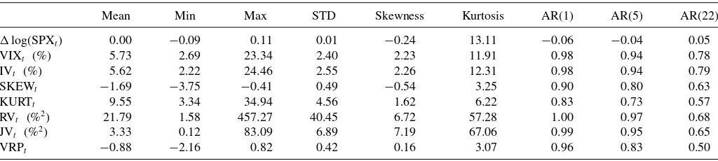
Table 2. Summary statistics
Mean Min Max STD Skewness Kurtosis AR(1) AR(5) AR(22)
log(SPXt) 0.00 −0.09 0.11 0.01 −0.24 13.11 −0.06 −0.04 0.05
VIXt (%) 5.73 2.69 23.34 2.40 2.23 11.91 0.98 0.94 0.78
IVt (%) 5.62 2.22 24.46 2.55 2.26 12.31 0.98 0.94 0.79
SKEWt −1.69 −3.75 −0.41 0.49 −0.54 3.25 0.90 0.80 0.63
KURTt 9.55 3.34 34.94 4.56 1.62 6.22 0.83 0.73 0.57
RVt (%2) 21.79 1.58 457.27 40.45 6.72 57.28 1.00 0.97 0.68
JVt (%2) 3.33 0.12 83.09 6.89 7.19 67.06 0.99 0.95 0.65
VRPt −0.88 −2.16 0.82 0.42 0.16 3.07 0.96 0.83 0.50
NOTE: The sample period covers January 1993 to December 2008;log(SPXt) refers to SPX log returns; VIXtis the VIX index, divided by√12 to get a monthly volatility measure for comparison; IVt, SKEWt, and KURTtdenote the 1-month option-implied volatility, skewness, and kurtosis, computed using the model-free approach of Bakshi, Kapadia, and Madan (2003); RVtand JVtare the realized volatility and the jump variation, respectively, calculated using 5-min high-frequency data over the past 22 trading days; VRPt≡log(RVt/VIX2
t) denotes the variance risk premium; and AR(i) means thei-lagged autocorrelation.
where is the sampling interval for the intraday data (we
use 5-min intervals). For each date t, we then sum the daily
realized volatilities over the previous month (rolling samples),
RVt ≡
21
i=0RV (d)
t−i, to get a monthly measure.
Following Carr and Wu (2009), we define the VRP as the log difference between monthly realized variance and
option-implied variance, VRPt ≡log(RVt/VIX2t),where VIXt is the
VIX index, divided by√12 to get a monthly volatility measure
comparable to RVt. We use the log difference because we find
that it provides a better measure than the difference in levels. A measure of jump risk is obtained using the approach of Barndorff-Nielsen and Shephard (2004). The bipower variation is given by
The daily jump variation is defined by subtracting the daily
bipower variation from the daily realized volatility, JV(td) ≡
max(RV(td)−BV
(d)
t ,0). And, finally, for each date t, we
sum the daily jump variations over the previous month, JVt ≡
21
i=0JV (d)
t−i, to get a monthly measure.
One- and three-month Treasury bill rates (obtained from the Federal Reserve website), interpolated to match option maturity, are used as a proxy for the risk-free rate. Dividend rates are ob-tained from the Standard and Poor’s information bulletin. Actual dividend payouts are used as a proxy for expected payouts.
Throughout, time is measured in trading days. SPX returns
and option-implied moments are plotted inFigure 1. Summary
statistics are reported inTable 2.
4.2 Parameter Estimates and Model Comparisons
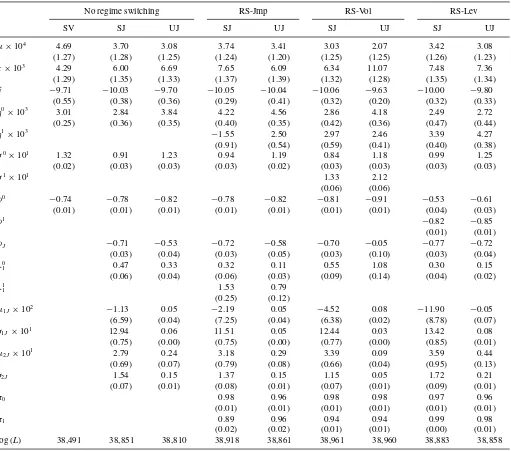
Parameter estimates and log-likelihoods for all of the models
under consideration are shown inTable 3. As found in previous
work, including jumps in returns and volatility gives a large improvement in log-likelihood relative to a model with no jumps (over 300 points in log-likelihood). We also looked at models with jumps in returns only, but these models work less well (including jumps in volatility is critical). The SJ model (jumps scaled by the volatility state) is strongly preferred over the UJ model (unscaled jumps). The improvement is over 40 points in
log-likelihood with the same number of parameters. In the scaled jump model, jumps are larger on average when volatility is high than when it is low, whereas in the unscaled jump model, jump sizes are identically distributed across time and unaffected by the volatility state. Although models with unscaled jumps have
been commonly used in previous work (e.g., Pan2002; Eraker,
Johannes, and Polson 2003; Broadie, Chernov, and Johannes
2007), this specification is not consistent with the data. Including the regime-switching feature in the model pro-vides additional large improvements. The SJ model with regime switching in volatility of volatility (SJ-RS-Vol) offers an im-provement of 110 points in log-likelihood relative to the cor-responding model without regime switching (SJ) at the cost of four additional parameters. Including regime switching in jump intensity (SJ-RS-Jmp) provides an improvement of 67 points in log-likelihood (relative to SJ), while including regime switch-ing in leverage effect (SJ-RS-Lev) provides a smaller but still important gain of 32 points in log-likelihood (relative to SJ).
A useful way to compare models is by using some form of information criterion. Akaike and Schwarz information criteria are common choices. These are based on comparison of log-likelihood minus some penalty based on the number of free parameters in the model. The Akaike information criterion uses a penalty equal to the number of free parameters, while the Schwarz criterion (also known as the Bayesian information cri-terion) uses a penalty equal to the number of free parameters
×ln(n)/2, wheren is the number of observations. For either
of these, the results are the same: SJ models are always pre-ferred over their UJ counterparts. For both SJ and UJ mod-els, the regime-switching variants are all preferred over their nonregime-switching counterparts. Among SJ models, the
rank-ing is SJ-RS-Vol≻SJ-RS-Jmp≻SJ-RS-Lev≻SJ. The
rank-ings are all decisive and provide strong evidence in favor of the regime-switching models. We note also that while the basic SJ model does not include regime switching, it does include jumps and is itself vastly better than the models with unscaled jumps (or no jumps at all) commonly used in the existing literature.
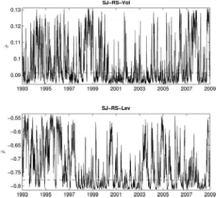
Time series plots of filtered values for the regime-dependent
parameters in several models are shown in Figure 3. For the
models with regime switching in volatility of volatility, for
ex-ample,σttakes on two possible values (σ0orσ1). The filter
de-scribed in Section3.2provides probabilities for each state
con-ditional on available information,ptj =p(st=j|Ft). Filtered
estimates ofσtare thus given by ˆσt =Et[σ(st)]=p0tσ0+p1tσ1
Table 3. Parameter estimates
No regime switching RS-Jmp RS-Vol RS-Lev
SV SJ UJ SJ UJ SJ UJ SJ UJ
µ×104 4.69 3.70 3.08 3.74 3.41 3.03 2.07 3.42 3.08
(1.27) (1.28) (1.25) (1.24) (1.20) (1.25) (1.25) (1.26) (1.23)
κ×103 4.29 6.00 6.69 7.65 6.09 6.34 11.07 7.48 7.36
(1.29) (1.35) (1.33) (1.37) (1.39) (1.32) (1.28) (1.35) (1.34)
v −9.71 −10.03 −9.70 −10.05 −10.04 −10.06 −9.63 −10.00 −9.80
(0.55) (0.38) (0.36) (0.29) (0.41) (0.32) (0.20) (0.32) (0.33)
η0
×103 3.01 2.84 3.84 4.22 4.56 2.86 4.18 2.49 2.72
(0.25) (0.36) (0.35) (0.40) (0.35) (0.42) (0.36) (0.47) (0.44)
η1 ×10³
−1.55 2.50 2.97 2.46 3.39 4.27
(0.91) (0.54) (0.59) (0.41) (0.40) (0.38)
σ0
×101 1.32 0.91 1.23 0.94 1.19 0.84 1.18 0.99 1.25
(0.02) (0.03) (0.03) (0.03) (0.02) (0.03) (0.03) (0.03) (0.03)
σ1
×101 1.33 2.12
(0.06) (0.06)
ρ0
−0.74 −0.78 −0.82 −0.78 −0.82 −0.81 −0.91 −0.53 −0.61
(0.01) (0.01) (0.01) (0.01) (0.01) (0.01) (0.01) (0.04) (0.03)
ρ1 −0.82 −0.85
(0.01) (0.01)
ρJ −0.71 −0.53 −0.72 −0.58 −0.70 −0.05 −0.77 −0.72
(0.03) (0.04) (0.03) (0.05) (0.03) (0.10) (0.03) (0.04)
λ0
1 0.47 0.33 0.32 0.11 0.55 1.08 0.30 0.15
(0.06) (0.04) (0.06) (0.03) (0.09) (0.14) (0.04) (0.02)
λ1
1 1.53 0.79
(0.25) (0.12)
µ1J×102 −1.13 0.05 −2.19 0.05 −4.52 0.08 −11.90 −0.05
(6.59) (0.04) (7.25) (0.04) (6.38) (0.02) (8.78) (0.07)
σ1J×101 12.94 0.06 11.51 0.05 12.44 0.03 13.42 0.08
(0.75) (0.00) (0.75) (0.00) (0.77) (0.00) (0.85) (0.01)
µ2J×101 2.79 0.24 3.18 0.29 3.39 0.09 3.59 0.44
(0.69) (0.07) (0.79) (0.08) (0.66) (0.04) (0.95) (0.13)
σ2J 1.54 0.15 1.37 0.15 1.15 0.05 1.72 0.21
(0.07) (0.01) (0.08) (0.01) (0.07) (0.01) (0.09) (0.01)
π0 0.98 0.96 0.98 0.98 0.97 0.96
(0.01) (0.01) (0.01) (0.01) (0.01) (0.01)
π1 0.89 0.96 0.94 0.94 0.99 0.98
(0.02) (0.02) (0.01) (0.01) (0.00) (0.01)
log (L) 38,491 38,851 38,810 38,918 38,861 38,961 38,960 38,883 38,858
NOTE: The sample period covers January 1993 through December 2008 (N=4025). Standard errors are in parentheses. Time is measured in trading days.
(t =1, . . . , n), with filtered estimates ˆρtand ˆλ1tcomputed anal-ogously.
In the regime-switching models, the states are quite persistent. With SJ-RS-Vol, for example, the estimated persistence
param-eters areπ0=0.98 andπ1=0.94 (the probability of staying in
regime 0 or regime 1, respectively, from one day to the next). The expected duration of stays is 50 days for regime 0 and 17 days for regime 1.
Expectations of future volatility of volatility and leverage ef-fect are dramatically different depending on the current regime. The estimated volatility of volatility parameters are 0.084 for state 0 versus 0.133 for state 1 in the SJ-RS-Vol model. The
es-timated leverage parameters are−0.53 for state 0 versus−0.82
for state 1 in the SJ-RS-Lev model. Because of the high degree of persistence in regime states, these differences remain even over relatively long time horizons. This is not of purely theoretical interest. Any investors interested in the dynamics of volatility will find this information useful. For example, volatility options
and swaps are highly dependent on the volatility of volatility. As discussed below, these persistent differences also affect the shape of the volatility smirk.
4.3 Diagnostics
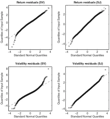
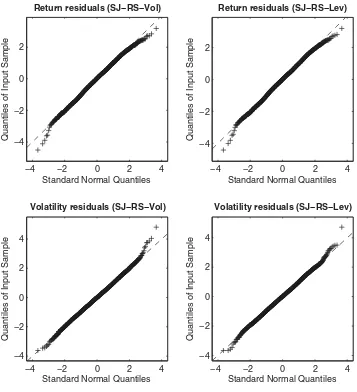
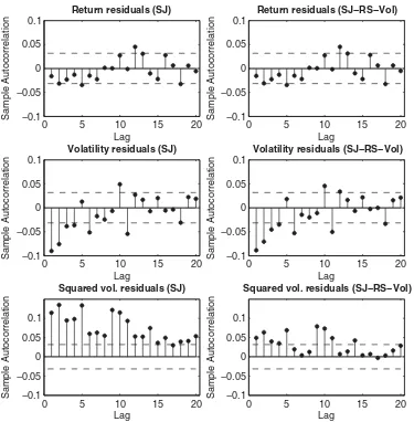
QQ-plots and correlograms for return and volatility residuals
are shown for several models in Figures4–6. Jarque–Bera and
Ljung–Box statistics are shown inTable 4.
The QQ-plots and Jarque–Bera statistics provide information regarding the extent to which the models are able to capture distributional characteristics of the data. Including jumps in the model provides an enormous improvement over the model with no jumps, consistent with the previous literature. This is true regardless of the form of the jumps (SJ or UJ). However, the scaled jump models (SJ) perform better than those with unscaled jumps (UJ), suggesting that they are better able to capture the nonnormality in return and volatility innovations observed in the
Figure 3. Time series of filtered values of state-dependent parameters. The dashed horizontal lines indicate the parameter estimates corre-sponding to the SJ model (which does not include regime switching in these parameters).
data. For the SJ models, including regime switching provides additional small improvements (for the UJ models, only regime switching in leverage effect helps much).
Turning now to the correlograms, all of the models do rel-atively well at eliminating autocorrelation in return residuals. On the other hand, all of the models fail with respect to the volatility residuals, which show significant negative autocorre-lation for the first several lags. This is suggestive of the exis-tence of a second volatility factor omitted by the model (e.g.,
Gallant, Hsu, and Tauchen 1999; Chacko and Viceira 2003;
Christoffersen, Heston, and Jacobs2009). All of the models also
show a large amount of unexplained autocorrelation in squared
volatility residuals. This is suggestive of stochastic volatility of volatility. Although the regime-switching model implements a very simple form of stochastic volatility of volatility, it is a substantial improvement over the other models (though still de-fective). Regime switching in jump intensity also helps some in this direction.
Note that since the generalized residuals are constructed using estimated model parameters, the standard asymptotics for the
test statistics reported in Table 4are not exact (see, e.g., Bai
2003for a discussion of this issue). However, the sample size
available to us is large, so parameter uncertainty would not be expected to have much impact. Monte Carlo studies that we have
Table 4. Diagnostic tests for generalized residuals
No regime switching RS-Jmp RS-Vol RS-Lev
SV SJ UJ SJ UJ SJ UJ SJ UJ
Jarque–Bera statistics
Return 445 20 113 19 117 17 245 10 50
(0.00) (0.00) (0.00) (0.00) (0.00) (0.00) (0.00) (0.01) (0.00)
Volatility 2,367 22 121 7 71 20 318 8 30
(0.00) (0.00) (0.00) (0.03) (0.00) (0.00) (0.00) (0.02) (0.00)
Ljung–Box statistics (20 lags)
Return 43 41 41 40 40 41 40 41 40
(0.00) (0.00) (0.00) (0.00) (0.00) (0.00) (0.00) (0.00) (0.00)
Volatility 116 118 116 113 111 115 100 115 114
(0.00) (0.00) (0.00) (0.00) (0.00) (0.00) (0.00) (0.00) (0.00)
Squared vol. 419 552 424 145 220 128 74 559 446
(0.00) (0.00) (0.00) (0.00) (0.00) (0.00) (0.00) (0.00) (0.00)
NOTE: Test statistics are shown withp-values in parentheses. The Jarque–Bera statistic is asymptoticallyχ2(2), implying a 5% critical value of 5.99. The Ljung–Box statistic is
asymptoticallyχ2(20), implying a 5% critical value of 31.41.
−4 −2 0 2 4 −6
−4 −2 0 2 4
Standard Normal Quantiles
Q
u
antiles of Inp
u
t Sample
Return residuals (SV)
−4 −2 0 2 4
−4 −2 0 2
Standard Normal Quantiles
Q
u
antiles of Inp
u
t Sample
Return residuals (SJ)
−4 −2 0 2 4
−4 −2 0 2 4 6
8
Standard Normal Quantiles
Q
u
antiles of Inp
u
t Sample
Volatility residuals (SV)
−4 −2 0 2 4
−4 −2 0 2 4
Standard Normal Quantiles
Q
u
antiles of Inp
u
t Sample
Volatility residuals (SJ)
Figure 4. QQ-plots for generalized residuals, SV and SJ models.
performed confirm that this is indeed the case. As discussed in
Section3.4, our primary interest here is using these diagnostics
as an aid in the process of model exploration. If one were more interested in formal specification testing, one might alternatively try applying tests such as those proposed by Bai (2003), Duan (2003), or Hong and Li (2005).
And finally, we note that while these diagnostics are useful in understanding directions in which the models are more or less successful in capturing various features of the data, and are informative in the process of model exploration, they do not provide a generically reliable basis for preferential ranking of the models. For this, a formal loss function is required (see, e.g.,
Diebold, Gunther, and Tay1998).
5. EXPLANATORY POWER FOR OPTION-IMPLIED SKEWNESS AND KURTOSIS
In this section, we examine whether the regime states implied by our regime-switching models have any explanatory power for the shape (e.g., third and fourth moments) of the risk-neutral distribution. Recall that option-implied skewness and kurtosis are not used in the estimation, which makes this diagnostic meaningful.
Given a model for the price of an asset and values for any rele-vant state variables, one can easily obtain the model-implied dis-tribution of returns at any horizon using Monte Carlo methods. We will refer to the third and fourth moments of these distribu-tions as model-implied skewness and kurtosis. Given time series for option-implied volatility and skewness (or kurtosis) and a model with two state variables (such as our regime-switching models), it is not difficult to find model parameters and values for the state variables such that model-implied and option-implied characteristics match exactly. To the extent that implied phys-ical and risk-neutral model parameters differ, these differences would typically be attributed to risk premia. However, since this approach confounds the information from physical dynamics and option prices, it is difficult to tell if the implied variation in states (e.g., leverage effect or volatility of volatility) is truly evident in the physical model or is just an artifact of trying to match the shape of the volatility smile. The problem here is a pervasive one in the option-pricing literature. It is possible to fit even a badly misspecified model to the data. The fitted model is likely to generate spurious risk premia, but the exact source and extent of the misspecification are difficult to diagnose.
The approach that we take in this article is different. While we match option-implied volatility exactly, we do not use the
−4 −2 0 2 4 −4
−2 0 2
Standard Normal Quantiles
Q
Standard Normal Quantiles
Q
Standard Normal Quantiles
Q
Standard Normal Quantiles
Q
Figure 5. QQ-plots for generalized residuals, SJ-RS-Vol and SJ-RS-Lev models.
information on option-implied skewness and kurtosis in the es-timation. In particular, we make no effort to use the information in option prices to come up with model parameters and regime states such that option-implied and model-implied skewness or kurtosis match exactly. We also do not look for risk premia that cause the models to fit the shape of the implied volatility smirk on average. Rather, we fit the models using only information from returns and implied volatility. We are then able to make a clear and unambiguous examination of the extent to which the implied states are informative about variation across time in observed option-implied skewness and kurtosis.
The idea is to regress option-implied skewness and kurtosis on the regime state, controlling for other possible determinants.
As described in Section3, it is not possible based on observed
data to determine the regime state conclusively. The available
information consists of filtered probabilities,pjt =p(st =j|Ft)
(j =0,1). The operational regression equations are thus
SKEWt =β0+β1sˆtRS-Vol+β2sˆtRS-Lev+β3sˆtRS-Jmp
t denote the filtered states
un-der the models with regime switching in volatility of volatility, leverage effect, and jump intensity, respectively [as defined in Equation (5)]. In interpreting the regression coefficients, note
that, for example, ˆst =0.30 implies that the probability that
st =1 conditional on data through timetis 30%. We also
in-clude several control variables: VIXt is the VIX index, which
serves as a proxy for the volatility state; and VRPt is the
vari-ance risk premium, which Bollerslev, Gibson, and Zhou (2011) argued reflects information on variation across time in investors’ risk aversion. Option-implied skewness and kurtosis may also be affected by the market expectation of jump risk. We proxy for
this by using a measure of realized jump variation, JVt. A more
detailed description of these variables may be found in Section 4.1. We first run the regressions on the control variables alone, and then add the regime states to the regressions to observe if there is a significant increase in explanatory power. We report
Newey–West robusttstatistics over eight lags (Newey and West
1987) and adjustedR2. For completeness, results are reported for the regressions based on filtered regime states from both SJ and UJ models.
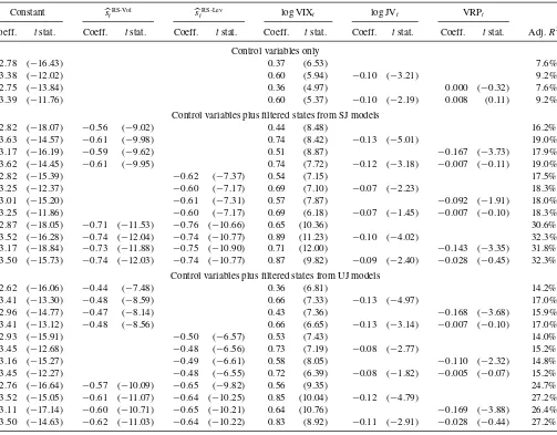
Table 5 shows the regressions for option-implied skew-ness. We first discuss the contributions of the control variables
0 5 10 15 20
Figure 6. Correlograms for SJ and SJ-RS-Vol models. Dotted lines show the 95% confidence band.
toward explaining option-implied skewness. The volatility state (VIX) is highly significant for all models and regardless of whether the regime state is included in the regression. The co-efficient is always positive, meaning that low volatility states are associated with more left-skewed return distributions. This is consistent with Dennis and Mayhew (2002), who reported a similar finding for individual stocks. Jump risk (JV) is also highly significant for all models. The coefficient is always neg-ative, suggesting that greater jump risk is associated with more left-skewed return distributions under the risk-neutral measure. This is consistent with intuition. In contrast, we do not find the VRP to be significant when the other control variables are included.
Although the volatility state is highly significant, it has rela-tively low explanatory power for option-implied skewness, with
an adjusted R2 of 7.6%. All of the control variables together
are able to explain only 9.2% of the time variation in option-implied skewness. This low explanatory power suggests that models with only a single state variable (volatility) will not be able to match time-varying patterns in the Black–Scholes volatility smirk realistically.
Including the filtered regime state in the regressions provides a dramatic improvement in explanatory power. SJ models al-ways outperform the corresponding UJ models. Including the
regime state from the models with regime switching in volatil-ity of volatilvolatil-ity (RS-Vol) is slightly better than including the regime state from the models with regime switching in leverage effect (RS-Lev). But the clear winner is the model that includes regime states from both of these. The states corresponding to volatility of volatility and regime switching each have substan-tial explanatory power when included in the regression alone. However, these two variables serve as complementary sources of information. For the regressions using states generated from the SJ models (together with all control variables), the adjusted
R2 is 18%–19% when either the RS-Vol or the RS-Lev states
are included individually, butR2jumps to over 32% when both
are included. The rankings here are consistent with the findings
reported in Sections4.2and4.3.
For the SJ-RS-Vol model (regime switching in volatility of volatility), the coefficient on the regime state is highly significant and in the expected direction. For the full regression (including regime state and all control variables), the estimated slope
co-efficient for the regime state is−0.61, indicating that a change
from state 0 to state 1 is associated with a 0.61 decrease in skewness (i.e., the distribution is substantially more left skewed
in the high volatility of volatility state). Thetstatistic is−9.95,
corresponding to a p-value of around 10−22. This model has
good explanatory power, with an adjustedR2of 19.0% (versus
Table 5. Regressions for option-implied skewness
Constant sRS-Vol
t s
RS-Lev
t log VIXt log JVt VRPt
Coeff. tstat. Coeff. tstat. Coeff. tstat. Coeff. tstat. Coeff. tstat. Coeff. tstat. Adj.R2
Control variables only
−2.78 (−16.43) 0.37 (6.53) 7.6%
−3.38 (−12.02) 0.60 (5.94) −0.10 (−3.21) 9.2%
−2.75 (−13.84) 0.36 (4.97) 0.000 (−0.32) 7.6%
−3.39 (−11.76) 0.60 (5.37) −0.10 (−2.19) 0.008 (0.11) 9.2%
Control variables plus filtered states from SJ models
−2.82 (−18.07) −0.56 (−9.02) 0.44 (8.48) 16.2%
−3.63 (−14.57) −0.61 (−9.98) 0.74 (8.42) −0.13 (−5.01) 19.0%
−3.17 (−16.19) −0.59 (−9.62) 0.51 (8.87) −0.167 (−3.73) 17.9%
−3.62 (−14.45) −0.61 (−9.95) 0.74 (7.72) −0.12 (−3.18) −0.007 (−0.11) 19.0%
−2.82 (−15.39) −0.62 (−7.37) 0.54 (7.15) 17.5%
−3.25 (−12.37) −0.60 (−7.17) 0.69 (7.10) −0.07 (−2.23) 18.3%
−3.01 (−15.20) −0.61 (−7.31) 0.57 (7.87) −0.092 (−1.91) 18.0%
−3.25 (−11.86) −0.60 (−7.17) 0.69 (6.18) −0.07 (−1.45) −0.007 (−0.10) 18.3%
−2.87 (−18.05) −0.71 (−11.53) −0.76 (−10.66) 0.65 (10.36) 30.6%
−3.52 (−16.28) −0.74 (−12.04) −0.74 (−10.77) 0.89 (11.23) −0.10 (−4.02) 32.3% −3.17 (−18.84) −0.73 (−11.88) −0.75 (−10.90) 0.71 (12.00) −0.143 (−3.35) 31.8% −3.50 (−15.73) −0.74 (−12.03) −0.74 (−10.77) 0.87 (9.82) −0.09 (−2.40) −0.028 (−0.45) 32.3%
Control variables plus filtered states from UJ models
−2.62 (−16.06) −0.44 (−7.48) 0.36 (6.81) 14.2%
−3.41 (−13.30) −0.48 (−8.59) 0.66 (7.33) −0.13 (−4.97) 17.0%
−2.96 (−14.77) −0.47 (−8.14) 0.43 (7.36) −0.168 (−3.68) 15.9%
−3.41 (−13.12) −0.48 (−8.56) 0.66 (6.65) −0.13 (−3.14) −0.007 (−0.10) 17.0%
−2.93 (−15.91) −0.50 (−6.57) 0.53 (7.43) 14.0%
−3.45 (−12.68) −0.48 (−6.56) 0.73 (7.19) −0.08 (−2.77) 15.2%
−3.16 (−15.27) −0.49 (−6.61) 0.58 (8.05) −0.110 (−2.32) 14.8%
−3.45 (−12.27) −0.48 (−6.55) 0.72 (6.39) −0.08 (−1.82) −0.005 (−0.07) 15.2%
−2.76 (−16.64) −0.57 (−10.09) −0.65 (−9.82) 0.56 (9.35) 24.7%
−3.52 (−15.05) −0.61 (−11.07) −0.64 (−10.25) 0.85 (10.04) −0.12 (−4.79) 27.2% −3.11 (−17.14) −0.60 (−10.71) −0.65 (−10.21) 0.64 (10.76) −0.169 (−3.88) 26.4% −3.50 (−14.63) −0.62 (−11.03) −0.64 (−10.22) 0.83 (8.92) −0.11 (−2.91) −0.028 (−0.44) 27.2%
NOTE: The table reports the results of the following regression:
SKEWt=β0+β1sˆRS-Volt +β2sˆtRS-Lev+β4log VIXt+ +β5log JVt+β6VRPt+εt.
Newey–West robusttstatistics over eight lags are shown in parentheses. The sample period covers January 1993 to December 2008; SKEWtdenotes the 1-month option-implied skewness. Filtered regime states are ˆsRS-Vol
t and ˆstRS-Levfor volatility of volatility and leverage effect, respectively. We also performed regression including the regime states from the RS-Jmp models; however, these were never significant. We do not report these results in the table to save space, but they are available upon request. The control variables are the VIX index, jump variation (JV), and variance risk premium (VRP). Results are shown for filtered states from both SJ (scaled jumps) and UJ (unscaled jumps) models.
9.2% for the control variables alone). These results are both statistically and economically significant.
Results for the SJ-RS-Lev model (regime switching in lever-age effect) are similar. In particular, the coefficient on the regime
state is highly significant and in the expected direction. Thet
statistic associated with this parameter is−7.17, corresponding
to ap-value of around 10−15. The model has an adjustedR2of
18.3%.
Table 6shows analogous regressions for option-implied kur-tosis. The results are qualitatively similar to those for option-implied skewness. The volatility state (VIX) is highly significant for all models and regardless of whether the regime state is in-cluded in the regression. The coefficient is negative, implying that low volatility states are associated with fatter-tailed return distributions. Jump risk (JV) is positively related to kurtosis. That is, the risk-neutral distribution tends to be more fat-tailed when jump risk is high, consistent with intuition. Although the VRP is highly significant when jump risk is omitted from the
regression, it has little explanatory power when jump risk is included.
Including the regime state in the regression provides ad-ditional improvement in explanatory power. As with option-implied skewness, SJ models always outperform the correspond-ing UJ models. Slope coefficients for the regime state have the expected signs. That is, higher volatility of volatility and stronger leverage effect are both associated with more kurtotic return distributions.
Including the regime state corresponding to regime switching in leverage effect is better here than including the regime state corresponding to regime switching in volatility of volatility
(ad-justedR2of 22.9% for SJ-RS-Lev vs. 18.1% for SJ-RS-Vol). As
is the case with implied skewness, including both regime states
in the regression is better yet, with anR2 of 25.8%. In the full
model, slope coefficients are 3.11 and 5.19 (withtstatistics of
5.52 and 8.66) for the SJ-RS-Vol and SJ-RS-Lev states, respec-tively. These are both economically and statistically significant.
Table 6. Regressions for option-implied kurtosis
Constant sRS-Vol
t s
RS-Lev
t log VIXt log JVt VRPt
Coeff. tstat. Coeff. tstat. Coeff. tstat. Coeff. tstat. Coeff. tstat. Coeff. tstat. Adj.R2
Control variables only
20.22 (12.46) −3.66 (−6.96) 8.4%
32.99 (13.34) −8.40 (−9.68) 2.02 (8.02) 16.6%
19.23 (11.34) −3.21 (−5.64) 0.02 (2.22) 8.7%
32.49 (13.23) −7.98 (−8.74) 1.72 (4.94) 0.65 (1.08) 16.7%
Control variables plus filtered states from SJ models
20.31 (12.67) 1.44 (2.44) −3.81 (−7.45) 9.0%
33.86 (14.27) 2.18 (3.90) −8.91 (−10.83) 2.14 (8.93) 18.0%
26.82 (14.40) 1.99 (3.49) −5.18 (−9.70) 3.03 (7.22) 15.5%
33.33 (14.19) 2.19 (3.93) −8.46 (−9.80) 1.82 (5.38) 0.70 (1.18) 18.1%
20.51 (12.11) 5.14 (7.03) −5.00 (−7.57) 16.2%
31.98 (13.75) 4.60 (7.13) −9.14 (−10.79) 1.82 (7.12) 22.8%
26.15 (14.73) 4.84 (7.30) −6.06 (−10.03) 2.65 (6.33) 21.2%
31.39 (13.39) 4.62 (7.16) −8.65 (−9.55) 1.47 (4.20) 0.76 (1.33) 22.9%
20.69 (12.63) 2.50 (4.31) 5.63 (8.11) −5.40 (−8.68) 18.0%
33.09 (15.13) 3.09 (5.47) 5.17 (8.60) −9.95 (−12.69) 1.96 (8.16) 25.6%
26.81 (15.80) 2.97 (5.22) 5.40 (8.74) −6.62 (−11.87) 2.86 (7.03) 23.8%
32.44 (14.75) 3.11 (5.52) 5.19 (8.66) −9.41 (−11.24) 1.57 (4.71) 0.85 (1.51) 25.8%
Control variables plus filtered states from UJ models
20.00 (12.07) 0.59 (1.07) −3.64 (−6.94) 8.5%
33.07 (13.62) 1.34 (2.64) −8.58 (−10.20) 2.12 (8.74) 17.3%
26.18 (13.80) 1.14 (2.19) −4.91 (−9.05) 2.99 (7.06) 14.8%
32.55 (13.52) 1.36 (2.68) −8.13 (−9.20) 1.80 (5.28) 0.69 (1.15) 17.4
21.47 (12.52) 4.21 (6.24) −5.00 (−7.85) 13.7%
33.56 (13.99) 3.91 (6.57) −9.43 (−10.79) 1.93 (7.63) 21.1%
27.40 (14.89) 4.08 (6.64) −6.16 (−10.24) 2.80 (6.73) 19.3%
32.99 (13.74) 3.93 (6.59) −8.95 (−9.73) 1.58 (4.56) 0.75 (1.32) 21.3%
21.01 (12.26) 1.54 (2.88) 4.63 (7.10) −5.09 (−8.34) 14.6%
33.79 (14.66) 2.25 (4.48) 4.49 (7.87) −9.89 (−12.00) 2.07 (8.58) 23.0%
27.21 (15.19) 2.10 (4.10) 4.64 (7.87) −6.36 (−11.31) 3.00 (7.33) 20.9%
33.16 (14.40) 2.27 (4.54) 4.52 (7.90) −9.35 (−10.81) 1.69 (5.06) 0.84 (1.48) 23.2%
NOTE: The table reports the results of the following regression:
KURTt=β0+β1sˆtRS-Vol+β2ˆstRS-Lev+β4log VIXt+β5log JVt+β6VRPt+εt.
Newey–West robusttstatistics over eight lags are shown in parentheses. The sample period covers January 1993 to December 2008. KURTtdenotes the 1-month option-implied kurtosis. Filtered regime states are ˆsRS-Vol
t and ˆstRS-Levfor volatility of volatility and leverage effect, respectively. We also performed regression including the regime states from the RS-Jmp models; however, these were never significant. We do not report these results in the table to save space, but they are available upon request. The control variables are the VIX index, jump variation (JV), and variance risk premium (VRP). Results are shown for filtered states from both SJ (scaled jumps) and UJ (unscaled jumps) models.
6. CONCLUSION
This article proposes a new class of models that layer regime switching on top of a standard stochastic volatility model with jumps in both returns and volatility. Motivated by the time-varying nature of option-implied skewness and kurtosis that is a prominent feature of observed data, we allow for regime switch-ing in three parameters of the basic model: volatility of volatil-ity, leverage effect, and jump intensity. All three parameters play important roles in determining the skewness and kurtosis of returns.
The application looks at SPX index and option data. In the first step of the analysis, we estimate the models relying only upon observations of the index price and option-implied volatility. This allows us to use observations on option-implied skewness and kurtosis for diagnostic purposes.
The models with regime switching fit the data dramatically better than those without regime switching. Accounting for time
variation in the volatility of volatility, leverage effect, or jump intensity not only increases log-likelihood significantly, but also provides improvements in other diagnostics of model fit.
While this first step of the analysis provides strong evidence of time variation in model characteristics that are related to the shape of return distributions under the physical measure, the second step investigates the relationship between these char-acteristics and the skewness and kurtosis of returns under the risk-neutral measure (i.e., implied by observed option prices). This part of the study is carried out by running regressions of option-implied skewness and kurtosis on the regime states ex-tracted in the estimation step (and several control variables).
We find that there is a strong relationship between model characteristics related to the shape of return distributions under the physical measure and the skewness and kurtosis of return distributions implied by option prices. Although commonly used models in the existing literature include volatility as the only
state variable, this variable has an adjustedR2of only 7.6% for
option-implied skewness. In contrast, regressions that include either the regime state corresponding to volatility of volatility or leverage effect (together with the control variables) have an
adjusted R2 of 18%–19%. When both states are included in
the regression, the adjustedR2is over 32%. Slope coefficients
on the regime states are highly significant and in the expected direction. Option-implied return distributions tend to be more left-skewed and leptokurtic when volatility of volatility is high or leverage effect is strong. Results for option-implied kurtosis are qualitatively similar though weaker.
We also find that the specification of jump distributions is important both in fitting the time-series data of returns and volatility and in explaining variation in option-implied skewness and kurtosis. Volatility-scaled jumps (SJ) outperform unscaled jumps (UJ) in both respects.
ACKNOWLEDGMENTS
We are grateful for the helpful comments and suggestions of Jonathan Wright (the editor), two anonymous referees, David Bates, Peter Chrisoffersen, Jakˇsa Cvitani´c, John Geweke, Kris Jacobs, Bjorn Jorgensen, Yujin Oh, Mike Stutzer, Pascale Valery, and seminar participants at the University of Colorado, HEC Montreal, Eastern Finance Association 2010 Annual Meetings, 2010 NBER Summer Institute Working Group on Forecasting and Empirical Methods, and Front Range Finance Seminar.
Disclaimer: The analysis and conclusions set forth are those of the authors and do not indicate concurrence by other members of the research staff or the Board of Governors.
[Received May 2011. Revised October 2012.]
REFERENCES
A¨ıt-Sahalia, Y., and Kimmel, R. (2007), “Maximum Likelihood Estimation of Stochastic Volatility Models,”Journal of Financial Economics, 83, 413– 452. [108,110]
A¨ıt-Sahalia, Y., and Lo, A. W. (1998), “Nonparametric Estimation of State-Price Densities Implicit in Financial Asset State-Prices,”Journal of Finance, 53, 499–547. [112]
Andersen, T., Bollerslev, T., Diebold, F., and Ebens, H. (2001), “The Distribution of Realized Stock Return Volatility,”Journal of Financial Economics, 61, 43–76. [112]
Andersen, T., Bollerslev, T., Diebold, F., and Labys, P. (2003), “Modeling and Forecasting Realized Volatility,”Econometrica, 71, 579–625. [112] Bai, J. (2003), “Testing Parametric Conditional Distributions of Dynamic
Mod-els,”Review of Economics and Statistics, 85, 531–549. [115]
Bakshi, G., and Kapadia, N. (2003), “Delta-Hedged Gains and the Negative Market Volatility Risk Premium,”Review of Financial Studies, 16, 527– 566. [110]
Bakshi, G., Kapadia, N., and Madan, D. (2003), “Stock Return Characteristics, Skew Laws, and Differential Pricing of Individual Equity Options,”Review of Financial Studies, 16, 101–143. [108,110,112]
Barndorff-Nielsen, O. E., and Shephard, N. (2002), “Econometric Analy-sis of Realized Volatility and Its Use in Estimating Stochastic Volatil-ity Models,”Journal of the Royal Statistical Society,Series B, 64, 253– 280. [112]
——— (2004), “Power and Bipower Variation With Stochastic Volatility and Jumps,”Journal of Financial Econometrics, 2, 1–37. [113]
Bollerslev, T., Gibson, M., and Zhou, H. (2011), “Dynamic Estimation of Volatility Risk Premia and Investor Risk Aversion From Option-Implied and Realized Volatilities,”Journal of Econometrics, 160, 235– 245. [110,117]
Broadie, M., Chernov, M., and Johannes, M. (2007), “Model Specification and Risk Premia: Evidence From Futures Options,”Journal of Finance, 62, 1453–1490. [109,113]
Carr, P., and Wu, L. (2007), “Stochastic Skew in Currency Options,”Journal of Financial Economics, 86, 213–247. [107]
——— (2009), “Variance Risk Premiums,”Review of Financial Studies, 22, 1311–1341. [110,112,113]
Chacko, G., and Viceira, L. (2003), “Spectral GMM Estimation of Continuous-Time Processes,”Journal of Econometrics, 116, 259–292. [115]
Chernov, M., and Ghysels, E. (2000), “A Study Towards a Unified Approach to the Joint Estimation of Objective and Risk Neutral Measures for the Purpose of Options Valuation,”Journal of Financial Economics, 56, 407–458. [110] Christoffersen, P., Heston, S., and Jacobs, K. (2009), “The Shape and Term Structure of the Index Option Smirk: Why Multifactor Stochastic Volatility Models Work So Well,”Management Science, 55, 1914–1932. [107,115] Christoffersen, P., Jacobs, K., and Mimouni, K. (2010), “Models for S&P500
Dynamics: Evidence From Realized Volatility, Daily Returns, and Option Prices,”Review of Financial Studies, 23, 3141–3189. [108]
Coval, J., and Shumway, T. (2001), “Expected Option Returns,”Journal of Finance, 56, 983–1009. [110]
Das, S. R., and Sundaram, R. K. (1999), “Of Smiles and Smirks: A Term Structure Perspective,”Journal of Financial and Quantitative Analysis, 34, 211–239. [107]
Dennis, P., and Mayhew, S. (2002), “Risk-Neutral Skewness: Evidence From Stock Options,”Journal of Financial and Quantitative Analysis, 37, 471– 493. [118]
Diebold, F., Gunther, T., and Tay, A. (1998), “Evaluating Density Forecasts With Applications to Financial Risk Management,”International Economic Review, 39, 863–883. [112,116]
Diebold, F., Hahn, J., and Tay, A. (1999), “Multivariate Density Forecast Eval-uation and Calibration in Financial Risk Management: High Frequency Returns on Foreign Exchange,”Review of Economics and Statistics, 81, 661–673. [112]
Duan, J.-C. (2003), “A Specification Test for Time-Series Models by a Normality Transformation,” Working Paper, University of Toronto. [116]
Eraker, B. (2004), “Do Equity Prices and Volatility Jump? Reconciling Evidence From Spot and Option Prices,”Journal of Finance, 59, 1367–1403. [109] Eraker, B., Johannes, M., and Polson, N. (2003), “The Impact of Jumps in
Volatility and Returns,”Journal of Finance, 58, 1269–1300. [109,113] Gallant, A. R., Hsu, C., and Tauchen, G. (1999), “Using Daily Range Data to
Calibrate Volatility Diffusions and Extract the Forward Integrated Variance,” Review of Economics and Statistics, 81, 617–631. [115]
Harvey, C. R., and Siddique, A. (1999), “Autoregressive Conditional Skewness,” Journal of Financial and Quantitative Analysis, 34, 465–487. [108] Heston, S. L. (1993), “A Closed-Form Solution for Options With Stochastic
Volatility With Applications to Bond and Currency Options,” Review of Financial Studies, 6, 327–343. [110]
Hong, Y., and Li, H. (2005), “Nonparametric Specification Testing for Continuous-Time Models With Applications to Term Structure of Interest Rates,”Review of Financial Studies, 18, 37–84. [116]
Jiang, G., and Tian, Y. (2007), “Extracting Model-Free Volatility From Option Prices: An Examination of the VIX Index,”Journal of Derivatives, 14, 35–60. [112]
Johnson, T. C. (2002), “Volatility, Momentum, and Time-Varying Skewness in Foreign Exchange Returns,”Journal of Business and Economic Statistics, 20, 390–411. [107]
Jones, C. (2003), “The Dynamics of Stochastic Volatility: Evidence From Underlying and Options Markets,” Journal of Econometrics, 116, 181– 224. [108]
Newey, W. K., and West, K. D. (1987), “A Simple Positive Semi-Definite, Het-eroskedasticity and Autocorrelation Consistent Covariance Matrix,” Econo-metrica, 55, 703–708. [117]
Pan, J. (2002), “The Jump-Risk Premia Implicit in Options: Evidence From an Integrated Time-Series Study,”Journal of Financial Economics, 63, 3–50. [110,113]
Santa-Clara, P., and Yan, S. (2010), “Crashes, Volatility, and the Equity Pre-mium: Lessons From S&P 500 Options,”Journal of Business and Economic Statistics, 92, 435–451. [107]