DSM ACCURACY EVALUATION FOR THE ISPRS COMMISSION I IMAGE MATCHING
BENCHMARK
G. Kuschka, P. d’Angeloa, R. Qinb, D. Polic, P. Reinartza, D. Cremersd
a
German Aerospace Center (DLR), Remote Sensing Technology Institute, 82230 Wessling, Germany -(georg.kuschk,pablo.angelo,peter.reinartz)@dlr.de
b
Singapore ETH Center, Future Cities Laboratory, CREATE Tower Singapore 138602 - [email protected] c
Terra Messflug GmbH, Eichenweg 42, 6460 Imst - [email protected] dTU Munich, Germany - [email protected]
Commission VI, WG VI/4
KEY WORDS:3D Stereo Reconstruction, DEM/DSM, Matching, Accuracy, Benchmark
ABSTRACT:
To improve the quality of algorithms for automatic generation of Digital Surface Models (DSM) from optical stereo data in the remote sensing community, the Working Group 4 of Commission I: Geometric and Radiometric Modeling of Optical Airborne and Space-borne Sensors provides on its websitehttp://www2.isprs.org/commissions/comm1/wg4/benchmark-test.htmla benchmark dataset for measuring and comparing the accuracy of dense stereo algorithms. The data provided consists of several optical spaceborne stereo images together with ground truth data produced by aerial laser scanning. In this paper we present our latest work on this bench-mark, based upon previous work.
As a first point, we noticed that providing the abovementioned test data as geo-referenced satellite images together with their corre-sponding RPC camera model seems too high a burden for being used widely by other researchers, as a considerable effort still has to be made to integrate the test datas camera model into the researchers local stereo reconstruction framework. To bypass this problem, we now also provide additional rectified input images, which enable stereo algorithms to work out of the box without the need for implementing special camera models. Care was taken to minimize the errors resulting from the rectification transformation and the involved image resampling.
We further improved the robustness of the evaluation method against errors in the orientation of the satellite images (with respect to the LiDAR ground truth). To this end we implemented a point cloud alignment of the DSM and the LiDAR reference points using an Iterative Closest Point (ICP) algorithm and an estimation of the best fitting transformation. This way, we concentrate on the errors from the stereo reconstruction and make sure that the result is not biased by errors in the absolute orientation of the satellite images. The evaluation of the stereo algorithms is done by triangulating the resulting (filled) DSMs and computing for each LiDAR point the nearest Euclidean distance to the DSM surface. We implemented an adaptive triangulation method minimizing the second order derivative of the surface in a local neighborhood, which captures the real surface more accurate than a fixed triangulation. As a further advantage, using our point-to-surface evaluation, we are also able to evaluate non-uniformly sampled DSMs or triangulated 3D models in general. The latter is for example needed when evaluating building extraction and data reduction algorithms.
As practical example we compare results from three different matching methods applied to the data available within the benchmark data sets. These results are analyzed using the above mentioned methodology and show advantages and disadvantages of the different methods, also depending on the land cover classes.
1. INTRODUCTION
Given the rising number of available optical satellites and their steadily improving ground sampling resolution, as well as ad-vanced software algorithms, large-scale 3D stereo reconstruction from optical sensors is increasingly getting a widespread method to cost-efficiently create accurate and detailed digital surface mod-els (DSMs). Their manifold usage includes for example monitor-ing of inaccessible areas, change detection, flood simulation / dis-aster management, just to name a few. Due to the amount of data, and with the prospect of a realtime global coverage by a network of optical satellites in the near future, the algorithms used for 3D stereo reconstruction have work fully automatic.
A natural engineering question for the development of these 3D stereo reconstruction algorithms is the availability of a common objective test-bed environment, comparing the stereo results with a known ground truth. In many computer vision related areas, such benchmarks boosted the development of their respective fields, as they directly allow to compare their numerical accuracy. In the area of 3D stereo reconstruction, the most prominent benchmarks
corre-sponding web page and thereby enable a objective online com-parison. We further simplified the first time usage of the data by providing rectified versions of the image data sets, thus en-abling participants to also run tests without having to care about the camera model. And additionally, we provide own results for two, now standard, dense stereo matching methods. These won’t be put into the official accuracy ranking, as we deem it unethical to provide a benchmark dataset, take care of the evaluation of its submissions, and at the same time participate in it.
2. BENCHMARK DATA
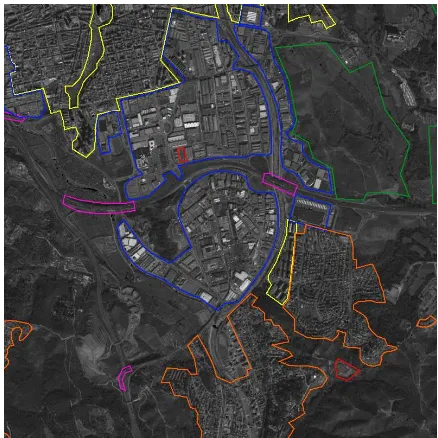
The publicly available optical satellite datasets used for the bench-mark were introduced in (Reinartz et al., 2010) and cover three characteristic sub-regions near Barcelona, Spain (see Figure1). To further investigate the accuracy of optical stereo reconstruc-tion methods in complex urban areas, one of these sub-regions (Terrassa) was manually classified into typical city areas like in-dustrial, residential, ... (see Figure2). For more detailled infor-mation on the satellite image acquisition properties as well as the reference data see (d’Angelo and Reinartz, 2011) and (Reinartz et al., 2010). All datasets and reference data is and will be provided at (ISPRS Satellite Stereo Benchmark, 2014), were all evalua-tions are and will be listed as well.
2.1 Datasets
Three datasets are part of the benchmark:
• Subsets of a Cartosat-1 Stereo pair, acquired in February 2008. It consists of a nadir viewing (−5◦
) and a forward viewing (+27◦
) scene. The ground sample distance is 2.5m.
• Worldview-1, one L1B stereo scene acquired in August 2008. One Nadir image (−1.3◦
) and one off-nadir scene (33.9◦ ), with ground sample distances of 0.5 and 0.76 meters.
• A Pleiades triplet, acquired on 8th of January 2013, with the following off nadir angles: forward image: 18◦
, nadir image:8◦
, and backward image:17◦ .
A RPC based block adjustment was performed, independently for each test area and sensor. GCPs derived from the ortho im-ages and LiDAR point cloud are used as reference, ensuring a good coregistration of the DSMs with the reference LiDAR point cloud. Both ortho images and LiDAR point clouds are provided by the Institut Cartogr`afic de Catalunya (ICC) - see Section2.2. For Cartosat-1, a 6-parameter affine RPC correction was used. For Worldview-1 and Pleiades, a row and column shift was suf-ficient. The corrections were applied to the RPCs, resulting in a good relative and absolute orientation of all datasets.
Benchmark participants can directly use the RPCs provided with the data without any further adjustment or correction with GCPs.
2.2 Reference Data
The reference data consist of color orthoimages with a spatial resolution of 50 cm as well as an airborne laser scanning point cloud (first pulse and last pulse) with approximately 0.3 points per square meter. The LiDAR points were acquired end of Novem-ber 2007.
Figure 1: Cartosat-1 image showing the three 4 km×4 km test areas: Terrassa, Vacarisses, La Mola
Figure 2: Cartosat-1 image showing the subareas in the urban ’Terrassa’ area. Blue: Industrial; Orange: Residential; Yellow: City; Purple: Bridges; Green: Open fields; Red: Changes
2.3 Epipolar rectification
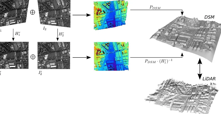
For enabling users to quickly test their stereo methods on our benchmark, we additionally provide rectified versions of the satel-lite images, allowing a 3D reconstruction by computing their dis-parity maps without having to deal with the RPC camera model. It should be noted that, although we provide a Windows binary for converting the computed disparity maps back into a UTM based DSM, the original satellite images and their RPC’s should be used to create DSMs with highest quality. The two ways of generating a DSM, either via RPCs or using the rectified images, are shown in Figure3.
The rigorous model of the linear push-broom sensors provides The International Archives of the Photogrammetry, Remote Sensing and Spatial Information Sciences, Volume XL-1, 2014
Figure 3: Two options to create the DSM, either with original satellite images and RPC camera model or using the rectified images. The triangulated DSM is then evaluated against the LiDAR ground truth
quasi-epipolar geometry for well-orientated images, where the search space of a point can be constrained to a curve in the search image. Due to the high stability of the spaceborne platform, this could be approximated as a straight line for data covering a rel-atively small area (Morgan et al., 2004), like in the case of our benchmark dataset. Therefore, the stereo images can be digitally rectified in a way that the matching correspondences are located on the same row of the rectified image grids, thus simplifying the matching problem and not needing the camera geometry anymore to produce a disparity map (Hartley and Zisserman, 2003). We adopt a two-step strategy for computing the rectified images, similar to the one proposed by (Wang et al., 2011). The basic idea of this approach is to first project the original images to a com-mon reference plane parallel to the ground, and then applying a 2D affine transformation to align the equivalent epipolar lines (EEL) to the same sampling row in the image grid. In most of the cases the RPC (Rational Polynomial Coefficient) are provided as a backward projection, namely from the object space to the image space, defined as
x=SampN um(X, Y, Z)
SampDen(X, Y, Z) , y=
LineN um(X, Y, Z)
LineDen(X, Y, Z) (1)
while the forward projection is computed iteratively by giving the height value. To rectify the projected images, we first need to find the pairs of EEL, which carry all the correspondence for each other. Simply put, the correspondences of points on the epipolar line in the left image can be found in its EEL on the right image. A pair of EEL can be computed with the following procedure: Given a point in the left image, we first compute its corresponding epipolar line in the right image (Zhao et al., 2008), and then based on the central point of this epipolar line, find its corresponding epipolar line back to the left image. These two lines are equiv-alent and contain the matching correspondences for each other. Given pairs of EEL, the transformation parameters for aligning these pairs of the EEL can be estimated by minimizing their er-rors in the vertical direction. We employ a 2D rigid transforma-tion for the image rectificatransforma-tion, which consists of rotatransforma-tion and translation. In practice, the 2D rigid transformation can be
calcu-lated by estimating the average rotation angles and y-axis offsets of the EEL pairs in a step-wise manner. The rotation angleθLfor the left image is computed as:
θl= 1
n
n
X
i
arcos(kl,i) (2)
wherekl,iis the slope of the epipolar lineiin the left image, and
nis the number of considered EELs. The angleθRfor the right image can be computed similarly. After applying the rotation to both images, the vertical shifttlandtrcan be estimated by taking the mean value of the vertical shifts of the rotated EEL:
tl= 1
n
n
X
i
(yr,i−yl,i) 2
tr=−tl (3)
where yl,i and yr,i are the vertical coordinates of the rotated EELs on the left and right images, respectively. The transfor-mation from the original imagesI to the rectified imageIrectcan be then described by the coordinate transformation
prect =A
p
1
= [Rθ T]
P
1
(4)
whereAis the affine transformation matrix containing the rota-tion matrixRθ∈R2×2with respect to the angle angleθ, plus the vertical translation vectorT=
0 t T
.
3. EVALUATION PROCEDURE
The automatic evaluation procedure requires the submitted DSMs to be projected into UTM Zone 31 North and sampled with two times the GSD (5m for Cartosat-1 and 1m for Worldview-1). Re-sulting holes need to be filled, otherwise a B-Spline based inter-polation method is used to fill remaining holes (Lee et al., 1997). In a first step, to ensure that the evaluation is not biased by errors in the orientation of the satellite images, the(x, y, z)-shift of the DSMs with respect to the reference point clouds is computed, us-ing an Iterative Closest-Point Algorithm (Besl and McKay, 1992) and the 3D-3D least-quares registration method of (Umeyama, 1991).
The final evaluation step is done by computing for each LiDAR point of the reference point cloud its distance to the meshed DSM surface. The LiDAR point is being projected onto the 2D grid of the corresponding DSM, falling between four incident pixels (x, y),(x+ 1, y),(x+ 1, y+ 1),(x, y+ 1). Instead of comparing the LiDAR height value with the interpolated height value of the DSM, we use a more robust distance measure and compute the minimum distance of the LiDAR point to the triangles created by the two possible triangulations of the DSM surface as shown in Figure4.
Figure 4: The two possible triangulations of a square involving four incident pixelsvijand the projected LiDAR point in blue.
As result, each LiDAR point from the reference data is associated with its distance to the computed DSM and the overall mean ab-solute error (MAE) per test area is computed. For the different sub-aeras of the datasetTerrassa(as shown in Figure2), masks
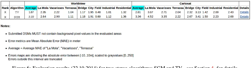
are applied to only evaluate the error inside these regions. For the final ranking of the algorithm’s accuracy, the average MAE over all sub-aeras is computed (compare Figure6).
To further give an intuitive feedback of the accuracy, locating ar-eas where algorithms perform quite well or bad, we also provide visual error maps as show in Figure5. For this purpose we project the LiDAR points (and their distances to the computed DSM re-spectively) onto a 2D grid, having the same geo-reference and ground sampling distance as the computed DSMs.
Figure 5: Evaluation of a sample area using the described ap-proach
4. DSM GENERATION
To provide first example results, we processed the benchmark data with two standard dense stereo matching methods, described in this section.
Let the image space of the reference image I1 be denoted as Ω ⊂ R2. For every pixelx = (x, y)T ∈ Ωand every height hypothesisγ∈Γ = [γmin, γmax], we compute a matching cost
C(x, γ)with respect to a second imageI2. The matching cost function is defined as
C(x, γ) =Dif f(Desc(I1,x), Desc(I2, π(x, γ)) ) (5)
withDescbeing a local image descriptor,πthe function project-ing a pixelx∈I1to imageI2by using the heightγ, andDif fa function to measure the difference of the aforementioned image descriptors.
As local image descriptorsDescwe used the Census transform (Zabih and Woodfill, 1994) with a9×7window, measuring their difference by the Hamming distance of their respective bit strings.
In the resulting three-dimensional(Ω×Γ)disparity space image (DSI), also called cost cube, we now search for a functionalu(x) (the disparity map), which minimizes the energy function arising from the matching costs (called data termEdata), plus additional regularization terms. As the data term is prone to errors due to some incorrect and noisy measurements, one often needs some smoothness constraintsEsmooth, forcing the surface of the dis-parity map to be locally smooth.
u(x) = argmin
This energy is non-trivial to solve, since the smoothness con-straints are based on gradients of the disparity map and therefore cannot be optimized pixelwise anymore. Various approximations for this NP-hard problem are existing, e.g. Semi-global Match-ing (Hirschmueller, 2005), energy minimization via graph cuts (Boykov et al., 2001) or minimization of Total Variation (Pock et al., 2008) - just to name three examples. When the matching costsCand the smoothness penalties∇uare normed, one can steer the smoothness of the resulting height map using a scalar balancing parameterλwithout the need to choose it manually, depending on the height values of the given data and there possi-ble gradients respectively.
4.1 Semi-global Matching (SGM)
In the work of (Hirschmueller, 2005), the energy functional of Equation6is approximated as follows
E(u) =X
The first term is the matching cost, the second and third term are penalties for small and large disparity discontinuities between neighboring pixelsp∈Nx. The parametersP1andP2serve as balancing parameter between the data term and the smoothness terms (similar toλin Equation6). The key idea is now not to solve the intractable global 2D problem, but to approximate it by combining 1D solutions from different directionsr, solved via dynamic programming
For details about how the aggregated costsLrare computed, the reader is referred to (Hirschmueller, 2005). In our results (Section The International Archives of the Photogrammetry, Remote Sensing and Spatial Information Sciences, Volume XL-1, 2014
5.), the penalties were set toP1 = 0.4andP2 = 0.8(with the raw costs normed to[0,1]).
4.2 Minimizing Total Variation (TV)
In a second approach we minimize the Total Variation of Equa-tion6using the primal-dual algorithm of (Pock et al., 2008).
u(x) = argmin u
Z
Ω
λ·C(x, u(x)) +∇u(x)dx
≈argmin u,a
Z
Ω
λ·C(x, a(x)) +∇u(x) + 1 2θ(u−a)
2
dx
(9)
In (Steinbruecker et al., 2009), a quadratic relaxation between the convex regularizer∇u(x)and the non-convex data termC(x, u(x)) was proposed for minimizing a Total Variation based optical flow energy functional and (Newcombe et al., 2011) used a similar approach for image driven and TV-based stereo estimation. We build upon these ideas and split the stereo problem from Equa-tion6into two subproblems and, using quadratic relaxation, cou-ple the convex regularizerR(u)and non-convex data termC(u) through an auxiliary variablea:
E=
Z
Ω
R(u) +λ·C(a) + 1 2θ(u−a)
2
dx . (10)
By iteratively decreasingθ→0, the two variablesu,aare drawn together, enforcing the equality constraintu=a. While the reg-ularization term is convex inuand can be solved efficiently us-ing a primal-dual approach for a fixed auxiliary variablea, the non-convex data term can be solved point-wise by an exhaustive search over a set of discretely sampled disparity values. This pro-cess is done alternatingly in an iterative way. For further details about the minimization procedure, the reader is referred to the work of (Pock et al., 2008), (Newcombe et al., 2011), (Kuschk and Cremers, 2013).
In our results (Section5.), the impact of the data term was set to
λ= 0.1(with the raw costs normed to[0,1]).
5. RESULTS
We provide initial results for two dense stereo matching meth-ods, which won’t be put into the official accuracy ranking. These two algorithms were described in the former section: SGM - Sec-tion4.1and a Variational approach - Section4.2. Except for the stereo algorithms themselves, all other parameters were fixed to the same settings (e.g. post-processing steps like median filtering and interpolation of holes due to UTM projection or the Census transform as image matching cost function).
No exhaustive parameter tuning was performed, and the parame-ters for the impact of the smoothness term were chosen in a way to provide a similar smoothness of the resulting DSMs. As image matching cost function, a simple Census Transform was chosen, see Section4..
6. CONCLUSIONS
In this work we improved and extended the existing ISPRS Stereo Benchmark. The submitted DSMs are evaluated for all three test areas and with respect to different land cover types as well. All
numerical and visual results will be displayed with the appli-cants consent on the corresponding web page and thereby enable a objective online comparison for the different algorithms. All datasets and reference data are publicly available and we heartily invite researchers in the field of 3D reconstruction from remote sensing imagery to evaluate their algorithms with the proposed benchmark. In a next step we plan to do a thorough evaluation of the state of the art image matching cost functions and the opti-mization methods for the energy functional to minimize.
ACKNOWLEDGMENT
Figure 6: Evaluation results (22.10.2014) for two stereo algorithms: SGM and TV - see Section4.for details.
REFERENCES
Besl, P. and McKay, N., 1992. A Method for Registration of 3-D Shapes. IEEE Transactions on pattern analysis and machine intelligence 14(2), pp. 239–256.
Boykov, Y., Veksler, O. and Zabih, R., 2001. Fast Approximate Energy Minimization via Graph Cuts. IEEE Transactions on pat-tern analysis and machine intelligence pp. 1222–1239. Graph Cuts.
d’Angelo, P. and Reinartz, P., 2011. Semiglobal Matching Re-sults on the ISPRS Stereo Matching Benchmark. Vol. 3819, pp. 79–84.
Geiger, A., Lenz, P. and Urtasun, R., 2012. Are we Ready for Autonomous Driving? The KITTI Vision Benchmark Suite. In: Computer Vision and Pattern Recognition (CVPR), 2012 IEEE Conference on, IEEE, pp. 3354–3361.
Haala, N., 2013. The Landscape of Dense Image Matching Al-gorithms. In: Photogrammetric Week 2013, Wichmann Verlag, pp. 271–284.
Hartley, R. and Zisserman, A., 2003. Multiple View Geometry in Computer Vision. Cambridge Univ Pr.
Hirschmueller, H., 2005. Accurate and Efficient Stereo Process-ing by Semi-Global MatchProcess-ing and Mutual Information. In: Com-puter Vision and Pattern Recognition, 2005. CVPR 2005. IEEE Computer Society Conference on, Vol. 2, IEEE, pp. 807–814.
ISPRS Satellite Stereo Benchmark, 2014. http://www2. isprs.org/commissions/comm1/wg4/benchmark-test. html[Online; Status 15-Oct-2014].
Kuschk, G. and Cremers, D., 2013. Fast and Accurate Large-scale Stereo Reconstruction using Variational Methods. In: ICCV Workshop on Big Data in 3D Computer Vision, Sydney, Aus-tralia.
Lee, S., Wolberg, G. and Shin, S., 1997. Scattered Data Inter-polation with Multilevel B-Splines. Visualization and Computer Graphics, IEEE Transactions on 3(3), pp. 228–244.
Morgan, M., Kim, K., Jeong, S. and Habib, A., 2004. Epipolar geometry of linear array scanners moving with constant velocity and constant attitude. ISPRS, Istanbul, Turkey.
Newcombe, R., Lovegrove, S. and Davison, A., 2011. DTAM: Dense Tracking and Mapping in Real-Time. In: Computer Vi-sion (ICCV), 2011 IEEE International Conference on, IEEE, pp. 2320–2327.
Pock, T., Schoenemann, T., Graber, G., Bischof, H. and Cremers, D., 2008. A Convex Formulation of Continuous Multi-Label Problems. Computer Vision - ECCV 2008 pp. 792–805.
Reinartz, P., d’Angelo, P., Krauß, T., Poli, D., Jacobsen, K. and Buyuksalih, G., 2010. Benchmarking and Quality Analysis of DEM Generated from High and Very High Resolution Optical Stereo Satellite Data. Vol. 3818, pp. 1–6.
Scharstein, D. and Szeliski, R., 2002. A Taxonomy and Evalu-ation of Dense Two-Frame Stereo Correspondence Algorithms. International journal of computer vision 47(1), pp. 7–42.
Steinbruecker, F., Pock, T. and Cremers, D., 2009. Large Dis-placement Optical Flow Computation without Warping. In: Com-puter Vision, 2009 IEEE 12th International Conference on, IEEE, pp. 1609–1614.
Umeyama, S., 1991. Least-Squares Estimation of Transforma-tion Parameters between two Point Patterns. Pattern Analysis and Machine Intelligence, IEEE Transactions on 13(4), pp. 376–380.
Wang, M., Hu, F. and Li, J., 2011. Epipolar resampling of linear pushbroom satellite imagery by a new epipolarity model. ISPRS Journal of Photogrammetry and Remote Sensing 66(3), pp. 347– 355.
Zabih, R. and Woodfill, J., 1994. Non-parametric Local Trans-forms for Computing Visual Correspondence. Computer Vision - ECCV 1994 pp. 151–158. census transform, rank transform.
Zhao, D., Yuan, X. and Liu, X., 2008. Epipolar line generation from ikonos imagery based on rational function model. Inter-national Archives of the Photogrammetry, Remote Sensing and Spatial Information Sciences 37(B4), pp. 1293–1297.