Full Terms & Conditions of access and use can be found at
http://www.tandfonline.com/action/journalInformation?journalCode=ubes20
Download by: [Universitas Maritim Raja Ali Haji] Date: 12 January 2016, At: 23:07
Journal of Business & Economic Statistics
ISSN: 0735-0015 (Print) 1537-2707 (Online) Journal homepage: http://www.tandfonline.com/loi/ubes20
Analytical Bias Reduction for Small Samples in the
U.S. Consumer Price Index
Ralph Bradley
To cite this article: Ralph Bradley (2007) Analytical Bias Reduction for Small Samples in the U.S. Consumer Price Index, Journal of Business & Economic Statistics, 25:3, 337-346, DOI: 10.1198/073500106000000639
To link to this article: http://dx.doi.org/10.1198/073500106000000639
Published online: 01 Jan 2012.
Submit your article to this journal
Article views: 35
Analytical Bias Reduction for Small Samples in
the U.S. Consumer Price Index
Ralph B
RADLEYU.S. Bureau of Labor Statistics, Washington, DC 20212 (bradley.ralph@bls.gov)
The U.S. Bureau of Labor Statistics (BLS) faces sample size constraints when computing its Consumer Price Index (CPI–U). The samples are not sufficiently large for the index to equal a true “fixed basket” price index. This study adjusts for this small-sample bias by estimating the second order of a stochastic expansion of the index. Unlike increasing sample size, this adjustment is inexpensive because it uses the same data used to compute the CPI–U. From the beginning of 1999 to the end of 2003, we estimate that 63% of the difference between the BLS superlative index (C–CPI–U) and the CPI–U is the result of finite-sample bias, and the other 37% is commodity substitution bias.
KEY WORDS: Jevons price index; Laspeyres price index; Stochastic expansions.
1. INTRODUCTION
Properly measuring inflation is an essential ingredient in refereeing U.S. economic policy debates, setting optimal con-tracts, guiding monetary policy, and determining the financing needs of all levels of government. Although the U.S. Consumer Price Index (CPI–U) is perhaps the most widely used national inflation measure, it has many shortcomings. This study looks at one source of bias in the CPI–U. To compute the CPI–U, the Bureau of Labor Statistics (BLS) takes many small samples, and these small samples induce an upward bias in the CPI–U.
The CPI–U is a two-stage index. In the second stage, the “all-items” CPI–U is computed as a weighted average of 8,018 subindexes called price relatives, orrelatives. A relative is a price index for a group of commodities or services (called items) within a metropolitan area (called area). There are 38 geographic areas, calledprimary sampling units (PSUs), and 211 items that generate 38×211=8,018 cells. The relatives are computed in the first stage. Examples of the so-calleditem– areasare apples in Boston, rental housing in Seattle, and so on. BLS is limited in the number of prices that it can collect for each item–area, and sample sizes as small as 1 can be used to compute a relative. The relative is a nonlinear moment of the collected prices, and whereas the relative asymptotically con-verges to its true value, BLS samples are not large enough to achieve this consistency. Therefore, the CPI–U is a weighted average of relatives that suffer from finite-sample bias.
This study proposes a low-cost method to reduce this finite-sample bias by using the same data used to compute the CPI–U. Although this method improves the accuracy of the CPI–U, it is not as good a solution as the more costly alternative of increas-ing the item–area’s sample size. Increasincreas-ing sample size not only will reduce bias, but also will eliminate the variance effects of sampling error. This low-cost bias-adjustment method is based on a second-order approximation and does not purge sampling error effects on the variance.
Finite-sample bias in the relative has been widely reviewed. Before 1998, all CPI–U relatives were Laspeyres-type indexes that were ratios of averages. Early studies used methods de-scribed by Cochran (1963), who he reviewed the finite-sample bias from ratio estimation. Studies using these methods to de-rive finite-sample bias for price indexes include those of Kish, Namboordi, and Pillai (1962) and McClelland and Reinsdorf (1997). After 1998, most of the CPI–U relatives changed from a
Laspeyres form to a geometric mean or Jevons form. Unlike the Laspeyres-type relatives, the finite-sample bias of the geomet-ric mean relative is systematically positive because of Jensen’s inequality.
This study commenced after the BLS switch to the geometric mean relative, unlike the earlier ones mentioned here. Because finite-sample bias from a geometric mean relative is no longer a problem of ratio estimation, here we do not use the ratio method of the earlier studies; instead, we adjust for finite-sample bias by using the second-order term in stochastic expansion of the relative around its true parameter value to adjust the price rela-tive. Our methods closely resemble those outlined by Hahn and Newey (2004) and Rilstone, Srivastava, and Ullah (1996). The basic intuition behind this analytical bias adjustment is that we are using a second moment of prices and the curvature of the index function as additional estimation information. Stochastic expansion theory is the starting point for bootstrap theory that adjusts for bias and improves confidence interval estimation with Edgeworth expansions (see Hall 1992). This idea is often used in other econometric problems, such as weak instrumental variables (Hahn and Hausman 2002) or correcting for bias in nonlinear panel data models (Hahn and Newey 2004). Analyti-cal bias adjustment is not the only method of finite-sample bias correction. In earlier work (Bradley 2001), a simulated boot-strap correction was done only for food and home fuel items. However, doing a simulated bootstrap correction on the entire set of samples requires 8,018 bootstraps per month. Even in today’s environment of high-speed chips, this is still computa-tionally intractable.
BLS uses three different methods to compute relatives. The most widely used method is the geometric mean. In this study, we estimate that 96% of the finite-sample bias adjustments in the CPI–U comes from the relatives computed by a geomet-ric mean. The other methods used to compute relatives are the Laspeyres and the sixth root of a Laspeyres for certain hous-ing items. Although houshous-ing has the largest expenditure weight in the CPI–U, it contributes very little to the finite-sample bias of the overall CPI, because the housing samples are relatively large, and there is, surprisingly, much less variance in rents than
In the Public Domain Journal of Business & Economic Statistics July 2007, Vol. 25, No. 3 DOI 10.1198/073500106000000639
337
in the price of other goods and services. Food and apparel are the two groups that contribute the most to the finite-sample bias of the CPI–U.
There are several sources of bias in the CPI; finite-sample bias is just one of them. Lebow and Rudd (2003) gave the most up-to-date and comprehensive review of the various sources of bias or measurement error. It is important that finite-sample bias in the CPI–U not be confused with commodity substitution bias occurring because the Laspeyres-type form of the upper-level CPI–U does not allow for commodity substitution across items when there is a change in the ratio of price relatives. Lebow and Rudd (2003) and Shapiro and Wilcox (1997) measured commodity substitution bias by taking the difference between the CPI–U and a superlative price index. Earlier work (Bradley 2001) and the present study show that this is not the correct measure of commodity substitution bias, because finite-sample bias makes the CPI–U a biased estimator for a Laspeyres or “fixed-basket” price index. In earlier work (Bradley 2001) and here, proof is given that some superlative indexes, such as the Törnqvist index, do not suffer from finite-sample bias in the same way as a Laspeyres index does. Thus the difference be-tween the CPI–U and a superlative index estimates the sum of two sources of bias: commodity substitution bias and finite-sample bias. Thus the overall bias estimates generated in these previous studies are not affected.
Significant substitution opportunities cannot be expected among all of the 8,018 item–areas. For instance, suppose that the price of bananas in Philadelphia increases; Philadelphia residents will not substitute any item sold in another city for bananas in Philadelphia. At best, there are a few other items within food in Philadelphia that they can substitute in response to the price increase in bananas. If consumers do not substi-tute for items outside their geographic reach, this means that if the price of any 1 of the 211 items increases, then at most they have substitution opportunities with only<3% of the remaining cells. (Because they can substitute only within the geographic area, this means that only 1/38≈3% of the 8,018 cells are available.) This study confirms that the true upper-level form is close to a Laspeyres form. Most substitution activity is perhaps occurring within the item–area cell. For example, if the price of a certain brand of cereal increases, then consumers usually will change to another brand of cereal.
Because of finite-sample bias, the CPI–U is greater than the true “fixed-basket” price index; however, our proposed adjust-ment method reduces this bias using the same data used to com-pute the index in the first place. Thus improving the CPI–U with this method is less expensive and easier than replacing it with a timely superlative index in which expenditure data must be up-dated every month. The best way to mitigate finite-sample bias and regular sampling error variance is to increase sample size; but this is also costly. If budgets are constrained, then it seems that analytical bias reduction is the second-best alternative.
Section 2 briefly describes the properties of the price rel-ative. It uses traditional first-order expansion to show consis-tency, then uses stochastic second-order expansions to approx-imate the finite-sample bias adjustment. It discusses why the same adjustments should not be made to the relatives for either an upper-level Törnqvist or geometric mean index. Finally, this section shows how to additively decompose both the CPI–U and
the bias-adjusted CPI–U into the major commodity groups (i.e., food, medical care, housing). Section 3 describes a Monte Carlo simulation that verifies the properties established in Section 2. Section 4 gives a reestimate of the CPI–U when the second-order term is used to analytically correct for finite-sample bias. Section 5 concludes.
2. CONSTRUCTION AND ADJUSTMENT OF THE PRICE RELATIVE
2.1 Basic Construction of the Relative and Its Asymptotic Values
The formula used to construct the price relative in the CPI–U depends on the item. If it is believed that consumers substitute within an item (e.g., breakfast cereal or boys’ apparel) then a geometric mean index is computed. For other items where there seem to be few substitution opportunities (e.g., hospital services or electricity), a Laspeyres-type index is used. The month-to-month price index for housing rent and the “rental equivalence” for homeowners is the sixth root of a Laspeyres index, where the denominator contains rents from the period 6 months before the current month.
Let item–areas be indexed byi, let the sample observations within an item–area be indexed byj, and let the month-year be indexed byt. Denote thejth collected price in item–areaiand periodtaspijt. For a sample ofni price quotes, the geometric mean price relative for item–areaiis
RGit=exp
ni
j=1
ln(pijt/pijt−1)/ni
. (1)
RGitis intended to be an estimate of the entire item–area index, plimni→∞RGit. Note that the formulas in (1), (4), and (6) are simplifications of the actual formulas used at BLS. These sim-plifications do not change the results of this study; a technical appendix showing the equivalence between the formulas in this article and the actual BLS formulas is available from the author. Write
µGit= plim
ni→∞ ni
j=1
ln(pijt/pijt−1)/ni
=E
ni
j=1
ln(pijt/pijt−1)/ni
. (2)
The finite-sample bias of the geometric mean is
BGit=E(RGit)−exp(µGit). (3)
Becauseni
j=1ln(pijt/pijt−1)/niis a linear average, its
expecta-tion equalsµGit. But from Jensen’s inequality, the finite-sample bias will be positive if this sample average has nonzero vari-ance.
The Laspeyres relative is computed as
RLit=
ni j=1pijt/ni
ni
j=1pijt−1/ni
. (4)
Bradley: Analytical Bias Reduction for Small Samples 339 index, the Laspeyres relative is not globally convex, and as a result, unlike the geometric mean index, the finite-sample bias of the Laspeyres,BLit=E(RLit)−µLit, is not always positive.
For the housing index, a sixth root of a 6-month index is cal-culated. LettingRHitdenote the housing relative, the month-to-month change is estimated as
RHit=
Its asymptotic value and bias are
µHit=
2.2 First-Order Expansion of the Relative
To establish the first-order asymptotics of the relative (or
√n
consistency), we use a first-order stochastic expansion. This method is the usual approach to establish the consis-tency and asymptotic normality of an estimator; for example, Hansen (1982) used this method to establish the asymptotic properties of the generalized method-of-moments estimator, and Amemiya (1985) used this method to establish the asymp-totic properties of the maximum likelihood estimator. Follow-ing Hansen (1982), throughout this article, we assume that all price variances are bounded, and that for alliands,{pijs}nj=i1 is iid acrossj. For the geometric mean index, we expandRGit aroundµGitto get
iid assumption, we use the Lindeberg–Levy central limit the-orem to conclude that √ni(nj=i1ln(pijt/pijt−1)/ni−µGit)
For the Laspeyres, we get the first-order approximation
RLit−µLit=
Using the same approach for the housing Laspeyres, and de-noting σit,t−6=cov(pijt,pijt−6), we get the following√ni
re-Although first-order asymptotic theory holds for estimated price indexes, in many cases ni is small, so the asymptotics are not attained. In the case of first-order expansion of (8), the smallniinduces the expected value of theOp(n−i 1)term to be strictly positive, because the exp(·)function is strictly convex in its argument, and Jensen’s inequality applies. The Laspeyres and the housing relatives are not strictly convex in their ar-guments, and thus the finite-sample bias is not systematically positive or negative.
2.3 An Adjustment Using the Second-Order Expansion of the Relative
One problem here is that the sample sizes for many item ar-eas are too small for the asymptotics outlined in Section 2.2 to hold. Consequently, we propose an analytical bias correction of the relative by estimating the term in the second-order expan-sion of the relative, then using this estimate to adjust the sample relative.
For the geometric mean relative, the second-order expansion ofRGitaroundµGitis
Passing the expectations operator through this expression re-sults in
Let µGit = jn=i1ln(pijt/pijt−1)/ni and σGit2 = var(ln[pijt/
HereσGit2 should not be confused with the variances ofRGit computed by BLS. The sample estimate of geometric mean bias correction is
BGit=(1/2)σGit2 exp(µGit)/ni, (13)
and the bias-adjusted geometric mean relative isRGit=RGit−
BGit. We can now state the following result, the proof of which is given in the Appendix.
Proposition 1. If (a) ln(pijt)is iid acrossjand (b)E(ln(pijt/
pijt−1)4) <∞, then there is a finiteγGit2 such thatn3i/2(BGit−
BGit)→N(0, γGit2 ), whereBGitis the true finite-sample bias as defined in (11).
Proposition 1 says something about the precision of the sam-ple estimate of the finite-samsam-ple bias. It converges more rapidly to its true value,BGit, than the sample relativeRGitconverges to exp(µGit). In this sense,BGitis a more precise estimator ofBGit thanRGitis of exp(µGit). This is as expected, because the true bias BGit converges to 0 more rapidly thanRGit converges to its population value. To understand the full effect of the bias-adjusted relative,RGit, we state the following decomposition:
√n
i(RGit−exp(µGit))
=√ni(RGit−exp(µGit))−√ni(BGit−BGit)−√niBGit
=Op(1)−Op(ni−1)−Op(n−i1). (14)
This shows that bothRGitandRGithave the same limiting distri-bution, which is what we want because the asymptotic distribu-tion of the finite-sample bias,BGit, degenerates to 0. However, for “small”ni,RGitandRGithave different means, because both
E(BGit)andE(BGit)are strictly >0. Therefore, for finite sam-ples,RGit is a more precise estimator for exp(µGit)thanRGit. The first term on the right side of (14) shows that adjusting the relative byBGitwill not purge the variance in the relative that comes from sampling error.
For the Laspeyres relative, we get the second-order expan-sion
passing the expectations operator through this expression yields:
The Laspeyres bias correction is approximated as
BLit= leads to the following result.
Proposition 2. If (a)pijt is iid acrossjand (b)E(p4ijt) <∞, then there is a finiteγLit2 such thatn3i/2(BLit−BLit)→N(0, γLit2). We can go through the same second-order expansion for the housing relative to get
2.4 Effects on the All-Items Index
The month-to-month “all-items” CPI–U based on the BLS samples is wHit−1are corresponding expenditure weights for periodt−1.
Define the “true population” CPI–U as
Rt= would get the unambiguous result that the “all-items” CPI–U has positive bias [E(Rt−Rt) >0]. LetN be the total number of item–area cells; if all of the relatives were computed by the geometric mean and the variance of the sample means for each relative were>0, then we would get plimN→∞Rt−Rt>0. But
Bradley: Analytical Bias Reduction for Small Samples 341
because of the relatives are not geometric means, we cannot get this unambiguous result. The bias-adjusted “all-items” index is
In the previous section, we showed that whereas bothRMitand
RMit=RMit−BMit (M= {G,L,H}) have the same asymptotic properties, for finite samples,RMit is a more precise estimator forRMit.
It might be concluded that we need to make the same bias-adjustment “plug in” for a superlative index such as a Törnqvist. But this is not correct. To show this, we start with a simplified Törnqvist functional form,
whereRit is the true price relative between periodstandt−1 for item–areaiandwit is its expenditure share weight, which is a simple average of expenditure shares in periodtandt−1. Suppose thatTtis estimated by
Tt= timated by geometric mean indexes with fixed sample sizes,
ni{i=1, . . . ,N}, that are sufficiently small so that var(Rit) >0 when all ni’s are fixed and all of the relatives are geomean. BLS publishes a “Törnqvist-type” index called the C–CPI–U. For the CPI–U and the C–CPI–U,N is 8,018. This is an ad-equate size for assuming that the asymptotic properties of a Törnqvist are satisfied.
The C–CPI–U is a Törnqvist-type index, but some of the rel-atives are not geometric means. Nonetheless, in the empirical section of this article (Sec. 4), we show that 96% of the finite-sample bias in the “all-items” CPI–U can be attributed to the geometric mean indexes. Thus plugging bias adjustments into the C–CPI–U will most likely induce a negative bias.
2.5 Additive Decomposition of the Indexes and Bias Adjustments
The “all-items” CPI–U is the upper chained index,
It=
After computing the bias adjustment, we calculate the bias-adjusted CPI–U index as to 1. The final period, denoted as T, is December 2003. Note that (26) is chained over time, and we have not accounted for any of the time series properties of the prices.
From here on, we drop theG,L, andHsubscripts so that the relative and the bias correction are nowRit andBit. There are eight major groups in the “all items” CPI–U. Each group is a set of similar items; for example, the food group includes the banana, meat, cereal, and diary items. These eight BLS groups, with the designated letter in parentheses denoting the set of all items within the group, are as follows:
Food and beverages (F), Housing (H), Apparel (A), Transportation(T), Medical care (M), Recreation (R), Education and communication (E), Other goods and services(G).
We letG= {F,H,A,T,M,R,E,G}denote the set of groups. Because different groups have different price distributions and sample sizes, it is useful to disaggregate both the indexes and the bias adjustments to determine how each group contributes to these statistics. Because the indexes in (25) and (26) are chained, additive decomposition of the “all-items” CPI–U bias adjustment into the eight groups is not straightforward. To find the percent contribution of each group to the average monthly indexes and bias adjustment over the T periods, we need the following proposition, which proven in the Appendix.
Proposition 3. Monthly average growth in the CPI–U and the bias-adjusted CPI–U is (IT)1/T−1 and(IT)1/T −1. The
As a corollary, we can state the following.
Corollary 1. The contribution toI1T/T−I1T/T by a groupJ∈
Gis
T
t=1
Rtm(Rt,I1T/T)
T
t=1m(Rt,I
1/T T )
−
Rtm(Rt,I1T/T)
T
t=1m(Rt,I1T/T)
×
i∈Jwit−1Bit
Rt−Rt
.
This allows us to additively decompose the total bias adjust-ment,I1T/T−I1T/T, into the contribution made by each group.
3. MONTE CARLO SIMULATION
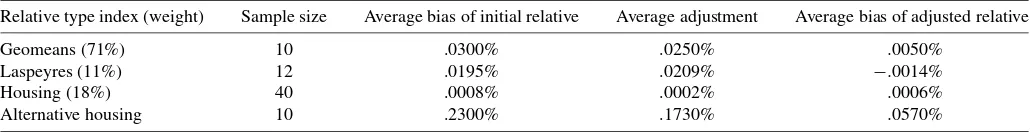
To verify the properties established in Section 2, we con-ducted a Monte Carlo experiment over a 12-month period. The parameters of this Monte Carlo experiment are calibrated to the published CPI–U. Historically, the average sample sizes for the geometric mean, Laspeyres, and housing relatives are 10, 12, and 40; thus in each of the 12 time periods, we draw re-peated samples of size 10 to compute rere-peated geomean rela-tives, of size 12 to compute repeated Laspeyres relarela-tives, and of size 40 to compute repeated housing relatives. Historically, the geomean, Laspeyres, and housing relatives have averaged 71%, 11%, and 18% of the expenditure weight in the “all-items” CPI–U. We use these upper-level weights in this experiment. The average variance of the month-to-month change in the log of prices is approximately .0025, and the annual CPI–U is close to 3%. In the Monte Carlo experiment, we sample the differ-ence in log prices from an iid N(.002463233, .0025), so that the mean compounded 12-month price growth is 3%. The true population relative for each period is then exp(.002463233). We repeat this process 2,000 times; this repetition is indexed asr. LetRM,t,r be the relative computed from theMth method (M=geomean, Laspeyres, housing), and letBM,t,rbe its corre-sponding bias adjustment computed from the sample moments. Table 1 reports the average of RM,t,r −exp(.002463233),
BM,t,r, and RM,t,r −exp(.002463233) in percentage terms (RM,t,r =RM,t,r−BM,t,r). Even though each of the methods faces the same data-generating process, the geomean has the largest bias. This cannot be explained entirely by sample size, because the sample size of the Laspeyres has only two more ob-servations, but the average bias is 35% less than the geomean. For the housing index, there is almost no bias. Therefore, the difference in functional form between the geomean and the Laspeyres plays a role in finite-sample bias. This provides evi-dence indicating that when BLS changed from a Laspeyres rela-tive to a geomean, finite-sample bias became a greater problem.
The geomean bias adjustment reduces the bias by 83%. The Laspeyres slightly overadjusts, and the housing correction is in-effective. Because there was so little bias in the housing relative, we decided to reinvestigate the housing adjustment by conduct-ing another simulation in which the sample size was 10 and the variance of the log of prices was increased to .64. We show the results in the row titled “Alternative housing.” Here the bias correction does perform better, but not as well as the geomean adjustment.
To investigate the impact of sampling error, Table 2 shows the performance of the estimated standard deviations of the log price for the geomeans and the price for both Laspeyres and housing. Because the difference in log prices is drawn from N(.002463233, .0025), the true standard deviation of the dif-ference of log of prices is√.0025=.05, and for prices it is
{exp(.00492t+.0050t)−exp(.00492t+.0025t)}1/2. Table 2 re-ports the results for the differences between the simulated stan-dard deviations and the true stanstan-dard deviations. As expected, the “Mean difference” column shows that the sample estimate is unbiased; however, the last three columns show that sampling error exists. In other words, on average we get the population standard deviation; however, for a particular sample there will be some error. For the geomean,>95% of the draws produce standard deviations in the interval(.045, .055), where the true standard deviation is .05, and although this does not allow for perfect bias adjustment, there is noticeable improvement. This provides evidence indicating that the bias-adjusted relative is a more precise estimator of the true relative than the unadjusted relative.
Finally, for each of the 2,000 repetitions, we compute an “all-items” yearly index by an expenditure weighted sum where the geomeans relative is given a 71% weight, the Laspeyres is given an 11% weight, and the housing is given a 18% weight. We do the same for the bias-adjusted relative. The average dif-ference between the unadjusted yearly index and the true in-dex is .34%, whereas the average difference between the bias-adjusted index and the true index is .09%. (These results closely resemble the results obtained using the actual BLS data base, as described in the next section.)
This experiment provides evidence that bias adjustment based on sample estimates of second-order approximations does not completely remove the bias. Sampling error remains a problem; however, this bias adjustment does greatly lower the bias.
4. RESULTS FOR THE CPI–U
We computed both the CPI–U (25) and the bias-adjusted CPI–U (26). Table 3 presents the annual and cumulative
re-Table 1. Simulation results: Finite-sample bias, the adjustment and bias for adjusted relative
Relative type index (weight) Sample size Average bias of initial relative Average adjustment Average bias of adjusted relative
Geomeans (71%) 10 .0300% .0250% .0050%
Laspeyres (11%) 12 .0195% .0209% −.0014%
Housing (18%) 40 .0008% .0002% .0006%
Alternative housing 10 .2300% .1730% .0570%
NOTE: These are the averages of 2,000 replications of 12-month draws. Using the notation of the text, the column labeled “Average bias of initial relative” is the mean ofRM,t,r−RM,t,r,
whereRM,t,r=exp(.002463), for allM,t,r. The column labeled “Average adjustment” is the average ofBM,t,r, and the last column reportsRM,t,r−RM,t,r.
Bradley: Analytical Bias Reduction for Small Samples 343
Table 2. Simulated difference between the sample standard deviations and the true standard deviations
Relative type Mean difference Standard deviation of difference Minimum difference Maximum difference
Geomenans −6.74E−05 .0023601 −.00494566 .020122428
Laspeyres 2.22E−06 .0011421 −.00250337 .008251568
Housing −8.06E−07 .000601 −.00177075 .003574577
NOTE: In this simulation, the difference in log prices is drawn from a N(.002463233t, .0025), wheretis the month number. Because the accuracy of the bias adjustment depends on the accuracy of the variance estimator, the table examines the distribution of the difference of the sample estimates of the variance and the true variance.
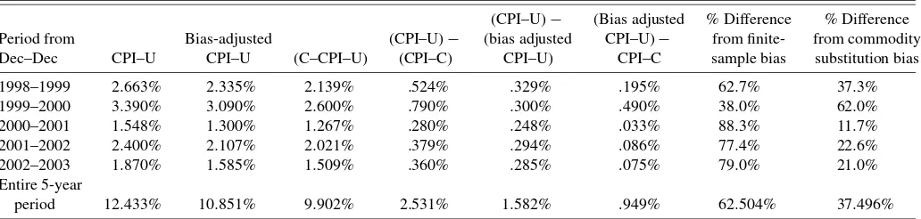
sults over the 60-month period from December 1998 to Decem-ber 2003. It also gives the results for BLS’s recently published “Törnqvist-type” index, the final C–CPI–U. The “(CPI–U−
C–CPI–U)” column gives the difference between the published CPI–U and the “Törnqvist-type” index. This difference fluctu-ates positively with the underlying inflation rate, ranging from .28% to .79%. The next columns decompose this difference between the difference of the CPI–U and the bias-adjusted in-dex and the difference between the bias-adjusted inin-dex and the C–CPI–U. The first difference can be attributed to finite-sample bias; the second difference may be attributed to commodity substitution bias. Over the 5-year period, these estimates at-tribute on average 62.5% of the difference between the pub-lished CPI–U and the C–CPI–U to finite-sample bias and the rest to commodity substitution bias. Because these estimates are based on second-order asymptotics, they do not completely eliminate bias. As mentioned earlier, we ignore the time series properties of the data when using the adjustment.
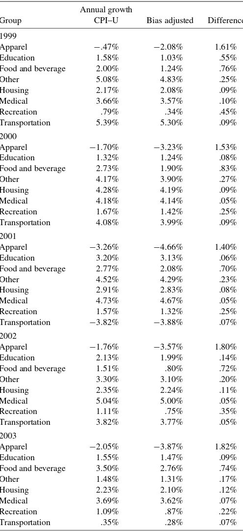
Table 3 gives the additive decompositions based on the method in Section 2.5. Table 4 lists the group contribution to the CPI–U, the bias-adjusted CPI, and the bias adjustment. Note that the group contribution to each of the indexes is the same; this occurs because there generally is very little difference be-tween the unadjusted and adjusted relatives. The round-off er-ror hides the slight difference. Although food and apparel con-tribute only 20.5% to the indexes, they concon-tribute 65.8% to the bias. This is because both food and apparel have unusually volatile prices, due in part to the frequency of sales. The bias for the geomean indexes is a positive function of the variance of the growth in the log of prices. Over the 5 years that this study was conducted, the average sample estimates of the variance of the growth log of prices for apparel, food, and transportation were .0028, .0016, and .00029. Table 5 lists the contribution
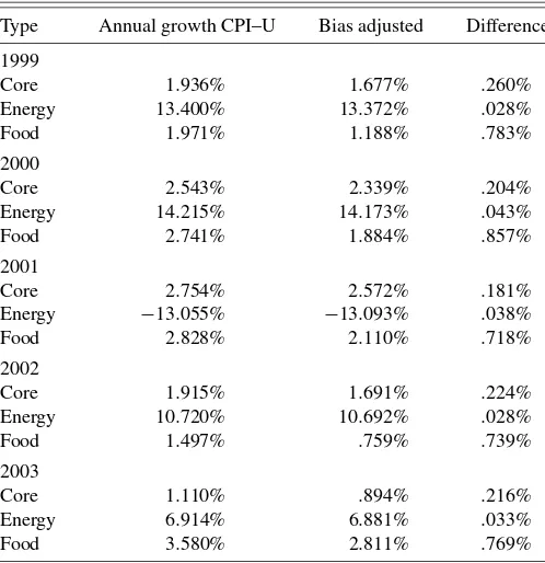
of the different methods. (Note that the housing group index is different from the housing relative method. The housing group includes home heating fuel, cleaning supplies, and various ser-vices; these items are not computed with the housing method.) From the result of the Monte Carlo simulation, it is not surpris-ing to find that 96% of the bias comes from the relatives based on the geomean method. Combining this result with the theo-retical results in Section 2.4 provides evidence indicating that “plugging in” bias-adjusted relatives into the C–CPI–U would induce additional bias. Table 6 breaks down the “all-items” in-dex into core and noncore parts. The core includes all items ex-cept non-alcohol–related food and beverages and energy items, such as motor and heating fuel. The purpose for the core in-dex is to remove items that are highly volatile over time but not necessarily volatile within an item–area. However, the volatility here is volatility over time rather than within an item area. The variances of the sample means for log prices of energy items are smaller because their sample sizes are larger. The average sample size for an energy item–area is 28, almost three times the sample size of a typical geomean index. Although energy prices fluctuate widely over time, there is relatively little price variation within time.
There is a large difference between a group’s contribution to the index and its contribution to the bias. This is because the bias adjustment varies widely by group. Looking at Table 7, the bias adjustment for apparel is the largest, whereas its share of the index is small. On the other hand, the bias adjustment for housing is smaller than average, whereas its share of the index is large. The food group is the largest contributor to the bias adjustment. Although its average bias adjustment is less than that of apparel, it has a higher expenditure share. Both the apparel and food group relatives are computed with geomean
Table 3. Summary statistics for the CPI–U, the bias-adjusted CPI–U, and the CPI–C
(CPI–U)− (Bias adjusted % Difference % Difference
Period from Bias-adjusted (CPI–U)− (bias adjusted CPI–U)− from finite- from commodity
Dec–Dec CPI–U CPI–U (C–CPI–U) (CPI–C) CPI–U) CPI–C sample bias substitution bias
1998–1999 2.663% 2.335% 2.139% .524% .329% .195% 62.7% 37.3%
1999–2000 3.390% 3.090% 2.600% .790% .300% .490% 38.0% 62.0%
2000–2001 1.548% 1.300% 1.267% .280% .248% .033% 88.3% 11.7%
2001–2002 2.400% 2.107% 2.021% .379% .294% .086% 77.4% 22.6%
2002–2003 1.870% 1.585% 1.509% .360% .285% .075% 79.0% 21.0%
Entire 5-year
period 12.433% 10.851% 9.902% 2.531% 1.582% .949% 62.504% 37.496%
NOTE: The column labeled “CPI–U” lists the 12-month growth in the published CPI–U. The column labeled “Bias-adjusted CPI–U” lists the 12-month change of the bias-adjusted CPI–U where the bias adjustment for the lower level geomeans relative is given in (13), the Laspeyres adjustment is given by (16), and the housing adjustment is given by (17). The column labeled “CPI–C” lists the 12-month growth in the BLS’s published chained CPI–C. The next three columns just list the differences in the first three. The last two columns lists the percent of the difference between the CPI–U and CPI–C comes from finite-sample bias and from substitution bias.
Table 4. Contributions to index growth and bias adjustment
Group Group Group
contribution contribution- contribution to
Group name CPI–U adjusted CPI–U bias adjustment
Apparel 4.5% 4.5% 25.6%
Education 5.5% 5.5% 3.1%
Food and beverage 16.0% 16.0% 40.2%
Housing 40.4% 40.4% 15.7%
Medical 5.8% 5.8% 1.2%
Recreation 6.0% 6.0% 6.2%
Transportation 17.3% 17.3% 4.4%
Other 4.6% 4.6% 3.5%
NOTE: The table lists the percent contribution to the cumulative 5-year growth rates for the CPI–U, the bias adjusted CPI–U, and the difference between the two. The decomposi-tion method is described in Proposidecomposi-tion 4.
indexes. Table 8 gives a yearly breakdown by core and non-core items. This shows the high “over-time” volatility of en-ergy, which contrasts with the relatively small “within-time” variability exhibited in Table 6.
5. CONCLUSIONS
The currently published CPI–U is an upward-biased estimate of a “fixed-basket” price index; therefore, the difference be-tween the CPI–U and a superlative index cannot be attributed entirely to commodity substitution bias. The CPI–U’s finite-sample bias can be reduced using the same data used to initially generate the index. Therefore, it is less costly.
On a year-to-year basis, it is not possible to predict the reduc-tion in the CPI–U if it is adjusted for finite-sample bias, but in the 5 years of this study, the CPI–U is reduced by .27% on aver-age. However, the bias adjustments are unpredictable, because they are based on the variance of prices within a cell, and these variances change unpredictably over time; they are also derived from a second-order approximation and thus do not completely eliminate bias, and their effectiveness in bias reduction depends on the time series properties of the collected prices.
Analytical bias reduction is not the only method that can be used to adjust for finite-sample bias, but it requires less compu-tation than bootstrapping and is less expensive than expanding sample sizes. However, if analytical bias reduction were imple-mented, then the final relatives that are used in the CPI–U would differ from those used in the C–CPI–U.
ACKNOWLEDGMENTS
The author thanks the referees, John Greenlees, Tim Erick-son, Ronald JohnErick-son, and Elliot Williams, for their feedback,
Table 5. Method type contributions to index growth and bias adjustment
Relative Type contribution Type contribution- Type contribution
type CPI–U adjusted CPI–U to bias adjustment
G 71.1% 71.1% 96.5%
L 17.7% 17.7% 2.5%
H 11.3% 11.3% 1.0%
NOTE: See the note for Table 4.
Table 6. Core type contributions to index growth and bias adjustment
Relative Type contribution Type contribution- Type contribution
type CPI–U adjusted CPI–U to bias adjustment
Core 77.8% 77.6% 59.7%
Energy 7.1% 7.1% .8%
Food* 15.3% 15.3% 39.8%
NOTE: See the note for Table 4.
Table 7. Annual growth in group indexes
Annual growth
Group CPI–U Bias adjusted Difference
1999
Apparel −.47% −2.08% 1.61%
Education 1.58% 1.03% .55%
Food and beverage 2.00% 1.24% .76%
Other 5.08% 4.83% .25%
Housing 2.17% 2.08% .09%
Medical 3.66% 3.57% .10%
Recreation .79% .34% .45%
Transportation 5.39% 5.30% .09%
2000
Apparel −1.70% −3.23% 1.53%
Education 1.32% 1.24% .08%
Food and beverage 2.73% 1.90% .83%
Other 4.17% 3.90% .27%
Housing 4.28% 4.19% .09%
Medical 4.18% 4.14% .05%
Recreation 1.67% 1.42% .25%
Transportation 4.08% 3.99% .09%
2001
Apparel −3.26% −4.66% 1.40%
Education 3.20% 3.13% .06%
Food and beverage 2.77% 2.08% .70%
Other 4.52% 4.29% .23%
Housing 2.91% 2.83% .08%
Medical 4.73% 4.67% .05%
Recreation 1.57% 1.32% .25%
Transportation −3.82% −3.88% .07%
2002
Apparel −1.76% −3.57% 1.80%
Education 2.13% 1.99% .14%
Food and beverage 1.51% .80% .72%
Other 3.30% 3.10% .20%
Housing 2.35% 2.24% .11%
Medical 5.04% 5.00% .05%
Recreation 1.11% .75% .35%
Transportation 3.82% 3.77% .05%
2003
Apparel −2.05% −3.87% 1.82%
Education 1.55% 1.47% .09%
Food and beverage 3.50% 2.76% .74%
Other 1.48% 1.31% .17%
Housing 2.23% 2.10% .12%
Medical 3.69% 3.62% .07%
Recreation 1.09% .87% .22%
Transportation .35% .28% .07%
NOTE: This table lists the December-to-December growth in the eight subindexes in the CPI–U. The column labeled “Bias adjusted” lists the growth of the bias adjusted CPI–U. It is important to note that Table 2 lists the contribution to the CPI–U whereas this table lists the subindexes.
Bradley: Analytical Bias Reduction for Small Samples 345
Table 8. Annual growth in core and noncore indexes
Type Annual growth CPI–U Bias adjusted Difference
1999
NOTE: This table lists the December-to-December growth rates in the core and noncore CPI–U and the bias-adjusted CPI–U.
and Uri Kogan for his careful proofing and review of the man-uscript. The views expressed here are solely those of the author and do not reflect either the policies or the procedures of the U.S. Bureau of Labor Statistics.
APPENDIX: PROOFS
Proof of Proposition 1
From (10), the following holds:
RGit−exp(µGit)
Passing through the expectations operator, we get
BGit=E[RGit−exp(µGit)] is bounded and because pGit is iid, we can use the Levy– Lindberg central limit theorem to conclude that there is aγGit2
such thatn3/2(BGit−BGit))) d
→N(0, γGit2 ).
The proof of Propositions 2 and 3 follow the same process and thus are omitted here.
Proof of Proposition 4
Reinsdorf, Diewert, and Ehemann (2002) showed that the index PG =ni=1(pit/pit−1)wi has the additive
decomposi-The within-month contribution of each item in the unadjusted and adjusted index is justwit−1Ritandwit−1Rit. BecauseBit=
Rit−Rit, we get the desired result.
[Received October 2004. Revised July 2006.]
REFERENCES
Amemiya, T. (1985),Advanced Econometrics, Cambridge, MA: Harvard Uni-versity Pres.
Biggeri, L., and Giommi, A. (1987), “On the Accuracy Precision of the CPI, Methods and Applications to Evaluate the Influence of Sampling House-holds,” in Proceedings of the 46th Session of the ISI, Tokyo, IP-12.1, pp. 137–154.
Boskin, M. J., Dulberger, E. R., Gordon, R. J., Griliches, Z., and Jorgensen, D. (1996), “Toward a More Accurate Measure of the Cost of Living: Final Re-port to the Senate Finance Committee for the Advisory Commission to Study the Consumer Price Index,” U.S. Senate Finance Committee.
Bradley, R. (2001), “Finite-Sample Effects in the Estimation of Substitu-tion Bias in the Consumer Price Index,”Journal of Official Statistics, 17, 369–390.
Cochran, W. G. (1963),Sampling Techniques(2nd ed.), New York: Wiley. Hahn, J., and Hausman, J. (2002), “A New Specification Test for the Validity of
Instrumental Variables,”Econometrica, 70, 163–189.
Hahn, J., and Newey, W. (2004), “Jacknife and Analytical Bias Reduction for Nonlinear Panel Models,”Econometrica, 72, 1295–1320.
Hall, P. (1992),The Bootstrap and Edgeworth Expansions, New York: Springer-Verlag.
Hansen, L. (1982), “Large-Sample Properties of Generalized Method-of-Moments Estimators,”Econometrica, 50, 1029–1054.
Kish, L., Namboordi, N. K., and Pillai, R. K. (1962), “The Ratio Bias in Sur-veys,”Journal of the American Statistical Association, 57, 92–115. Lebow, D., and Rudd, J. (2003), “Measurement Error in the Consumer Price
Index: Where Do We Stand?”Journal of Economic Literature, 41, 159–201. McClelland, R., and Reinsdorf, M. (1997), “Small-Sample Bias in the Geomet-ric Mean Seasoned CPI Component Indexes,” manuscript, Bureau of Labor Statistics.
Reinsdorf, M. B., Diewert, E. W., and Ehemann, C. (2002), “Additive Decom-position for Fisher, Törnqvist and Geometric Mean Indexes,”Journal of Eco-nomic and Social Measurement, 28, 51–61.
Rilstone, P., Srivastava, V. K., and Ullah, A. (1996), “The Second-Order Bias and Mean Squared Error of Nonlinear Estimators,”Journal of Econometrics, 75, 369–395.
Shapiro, M. G., and Wilcox, D. W. (1997), “Alternative Strategies for Aggre-gating Prices in the CPI,”Review of the Federal Reserve Bank of St. Louis, 113–125.