A multi-component, multi-species model of
vegetation–atmosphere CO
2
and energy exchange
for mountain grasslands
G. Wohlfahrt
a,b,∗, M. Bahn
a, U. Tappeiner
a,c, A. Cernusca
a aInstitut für Botanik, Universität Innsbruck, Sternwartestr. 15, 6020 Innsbruck, AustriabCentro di Ecologia Alpina, Viote del Monte Bondone, 38040 Trento, Italy cEuropäische Akademie Bozen, Domplatz 3, 39100 Bolzano, Italy
Received 3 April 2000; received in revised form 31 August 2000; accepted 18 September 2000
Abstract
A model is presented which allows simulation of vegetation–atmosphere CO2and energy exchange of multi-component,
multi-species canopies, explicitly taking into account the structural and functional properties of the various components and species. The model is parameterised for a meadow and an abandoned area at the ECOMONT study area Monte Bondone (1500 m a.s.l., Trento/Italy). A series of sensitivity tests showed the model to be sensitive to vegetation optical and physiological properties, but not to soil optical properties, dwarf shrub bole respiration parameters and phytoelement inclination and width. Validation of canopy CO2 and energy exchange rates against the respective fluxes measured by the means of the
Bowen-ratio-energy-balance method yields broadly satisfactory results. Though it proves difficult to validate canopy latent and sensible heat flux, due to the fact that the vegetation–atmosphere-transfer model does not include contributions by the soil, whereas measured fluxes do, indicating both the need for further model development as well as experimental studies. Finally, the model is used to test for the effects of simplifications in input data likely to occur when being applied at larger spatial and/or temporal scales. © 2001 Elsevier Science B.V. All rights reserved.
Keywords: Photosynthesis; Energy balance; Evapotranspiration; Mountain grassland; VAT
1. Introduction
The rates at which CO2 and energy are exchanged between the biosphere and atmosphere continues to be a subject of active research, motivated by fun-damental environmental changes occurring on our planet (e.g. Steffen et al., 1998; Lloyd, 1999; Running et al., 1999). In order to arrive at an understanding
∗Corresponding author. Present address: Institut für Botanik,
Universität Innsbruck, Sternwartestr. 15, 6020 Innsbruck, Austria. Tel.:+43-512-507-5917; fax:+43-512-507-2975.
E-mail address: [email protected] (G. Wohlfahrt).
of the processes controlling biosphere–atmosphere exchange, modelling studies play an important role, since model simulations allow to test future scenar-ios, to separate various component processes, and to study their interaction (Ehleringer and Field, 1993; Van Gardingen et al., 1997; Cernusca et al., 1998).
Two major approaches of representing the vege-tation component of the land surface may be dis-tinguished (Raupach and Finnigan, 1988): one line of models treats the vegetation as if it was a single “big leaf”, possibly distinguishing between a sunlit and a shaded fraction (De Pury and Farquhar, 1997; Wang and Leuning, 1998; Kellomäki and Wang, 1999;
Nomenclature
A net photosynthesis (mmol m−2s−1) AC canopy net photosynthesis (mmol m−2s−1) Bl normalised view factor (–)
Bu zonal distribution of scattered and emitted radiation (–) BREB Bowen-ratio-energy-balance method
cp specific heat of dry air (1010 J kg−1K−1) Ca CO2concentration of ambient air (mmol mol−1)
Ci CO2concentration in the intercellular space (mmol mol−1) Cs CO2concentration at the leaf surface (mmol mol−1)
CRY cryptogams
DgS, DngS green and non-green stems of dwarf shrubs DL dwarf shrub leaves
ea air water vapour pressure (hPa)
es(T) saturated leaf water vapour pressure (hPa) fsl fraction of sunlit phytoelements (–) F phytoelement inclination distribution (–) FC CO2flux above the canopy (mmol m−2s−1) FL, FS forb leaves and stems, respectively
FRU fruits
gbv all-sided boundary layer conductance to water vapour (mmol m−2s−1) gmin minimum stomatal conductance to water vapour (mmol m−2s−1) gsv stomatal conductance to water vapour (mmol m−2s−1)
gtv total conductance to water vapour (mmol m−2s−1) GAI green area index (m2m−2)
G(β,λ) projection of leaves with inclinationλinto inclinationβ(–) Gfac stomatal sensitivity coefficient (–)
GCM global circulation model
GL, GS graminoid leaves and stems, respectively hs leaf surface relative humidity (–) H sensible heat loss (W m−2) 1Ha energy of activation (J mol−1) 1Hd energy of deactivation (J mol−1)
Ifac coefficient representing the extent to which Rdark is inhibited in the light (–) INF inflorescences
IR long-wave radiation (W m−2) j subscript indicating canopy layer
L long-wave radiation incident on phytoelements (W m−2) 1L PAI in canopy layer (m2m−2)
Ld downward flux of long-wave radiation (W m−2) Le emitted long-wave radiation (W m−2)
Lu upward flux of long-wave radiation (W m−2) LAI leaf area index (m2m−2)
np number of species
NEC attached dead plant material NIR near infrared radiation (W m−2)
Oi O2concentration in the intercellular space (mmol mol−1) p subscript indicating species
Pi probability of interception (–)
Pml potential rate of RuBP regeneration (mmol m−2s−1) PAI plant area index (m2m−2)
PPFD photosynthetic photon flux density (mmol m−2s−1) Qd downward flux of diffuse short-wave radiation (W m−2) Qdir downward flux of beam radiation (W m−2)
Qshade short-wave radiation incident on shaded phytoelements (W m−2) Qsolar incident short-wave radiation (W m−2)
Qsun short-wave radiation incident on sunlit phytoelements (W m−2) Qu upward flux of diffuse short-wave radiation (W m−2)
R universal gas constant (8.314 m3Pa mol−1K−1)
Rabs bi-directional absorbed short-wave and long-wave radiation (W m−2) Rbole bole respiration (mmol m−2s−1)
Rdark dark respiration rate (mmol m−2s−1)
Rday respiration rate during day light (mmol m−2s−1) RN net radiation(soil+vegetation)(W m−2)
RNveg vegetation net radiation (RN−soil net radiation) (W m−2) Rsoil soil respiration (mmol m−2s−1)
RUBISCO ribulose-1,5-bisphosphate carboxylase/oxygenase RuBP ribulose-1,5-bisphosphate
S soil heat flux (W m−2) 1S entropy term (J K−1mol−1) Ta air temperature (◦C)
Tp phytoelement temperature (◦C) TpK phytoelement temperature (K)
TpKsh phytoelement temperature of shaded leaves (K) TpKsl phytoelement temperature of sunlit leaves (K) Tref reference temperature (273.16 K)
Ts soil surface temperature (◦C) TsK soil surface temperature (K)
VCmax maximum rate of carboxylation (mmol m−2s−1) VAT vegetation–atmosphere-transfer
WC RuBP-saturated rate of carboxylation (mmol m−2s−1) WJ RuBP-limited rate of carboxylation (mmol m−2s−1) Greeks
α apparent quantum yield of A at saturated CO2(mol CO2per mol photons) β angle of incidence (rad)
β∗ angle of the sun (rad)
γ psychrometric constant (Pa K−1)
δ Boolean variable indicating whether leaves are hypo- or amphistomatous (–) εc phytoelement thermal emissivity (–)
λ phytoelement angle (rad)
ξ reflection–transmission distribution function (–) ρ density of dry air (kg m−3)
ρc phytoelement reflection coefficient (–) ρs soil reflection coefficient (–)
σ Stefan–Boltzmann constant (5.67×10⁻⁸W m−2K−4) τ RUBISCO specificity factor (–)
τc phytoelement transmission coefficient (–)
Chen et al., 1999). Such models, given their reduc-tionist nature, are of use if computational efficiency is given preference over numerical accuracy, as it is in meso-scale or global climate (GCM) model appli-cations (Berry et al., 1998; Raupach et al., 1997; Cox et al., 1998; Anderson et al., 2000). A second line of models, often referred to as multi-layer models, retains the vertical profile of canopy structure and calculates micrometeorology and fluxes separately for each layer (e.g. Goudriaan, 1977; Tenhunen et al., 1994; Leuning et al., 1995; Baldocchi and Meyers, 1998; Tappeiner and Cernusca, 1998). These models represent useful tools for analysing the details of canopy CO2 and energy exchange processes.
The overwhelming complexity of many natural and semi-natural canopies, though, places formidable practical problems, which has led to a variety of approaches, reflecting the respective scientific per-spective. For example, many models consider the canopy to be composed solely of leaves, ignoring the existence of supporting structures (stems, twigs and branches), reproductive organs (inflorescences, fruits) and attached dead plant material (cf. Wenhan, 1993). This is manifested in the loose use of the term LAI (leaf area index), instead of PAI (plant area index), for the total above-ground silhouette area. Given the differing structural and functional properties of the various canopy components, it is clear that they con-tribute in different manners to whole canopy exchange processes. For example, dry dead plant material, as opposed to green matter, may dissipate absorbed energy solely via long-wave emission and sensible heat exchange (Paw U, 1987), and hence does not contribute to the canopy latent heat flux (Anderson
et al., 2000). In multi-species canopies, this issue be-comes even more complicated, since within each of the various canopy components several species must be distinguished, which are likely to be characterised by different structural and functional properties (Ten-hunen et al., 1994; Tappeiner and Cernusca, 1998; Sinoquet et al., 2000).
Semi-natural mountain grasslands fall both into the multi-component, as well as the multi-species category (Cernusca and Seeber, 1981; Tappeiner and Cernusca, 1994, 1995, 1996). These grasslands are often situated in the transition zone between the forest and the natural grasslands above the tree line, being created centuries ago by human activity (Spatz et al., 1978). The tran-sitional character and sustainable management made them highly diverse ecosystems, populated by a large number of different plant species (Tasser et al., 1999). The various species follow different temporal strate-gies (Bahn et al., 1994), so that at almost any instant during the vegetation period we will find species at different stages of their life cycle, e.g. vigorous veg-etative growth, flowering, fruiting, senescence. This strong variability also shows up in inter-specific dif-ferences with regard to gas exchange characteristics (Bahn et al., 1999; Wohlfahrt et al., 1999).
canopy CO2and energy exchange. Finally, by consid-ering the effects of simplifications in the input data likely to occur at larger spatial and/or temporal scales the applicability of the model at these larger scales will be assessed.
2. Materials and methods
2.1. Site
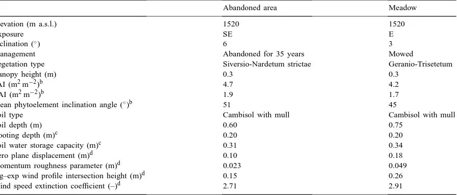
Field investigations were carried out within the frame of the EU-TERI-project ECOMONT during the summers of 1996–1998 in the Southern Alps on the Monte Bondone plateau (Trentino/Italy, latitude 46◦01′20′′N, longitude 11◦02′30′′E) at an elevation between 1500 and 1600 m above sea level. The mean annual temperature is 5.5◦C ranging from−2.7◦C in January to 14.4◦C in July (Gandolfo and Sulli, 1993). Precipitation is abundant throughout the whole year (1189 mm), with two peaks in June (132 mm) and October (142 mm) and a minimum of 53 mm in Jan-uary (Gandolfo and Sulli, 1993). Two sites, differing in land-use, were investigated: a hay meadow, mowed once a year, and an area abandoned 35 years ago. A
Table 1
General characterisation of the investigated sites at the Monte Bondone study areaa
Abandoned area Meadow
Elevation (m a.s.l.) 1520 1520
Exposure SE E
Inclination (◦) 6 3
Management Abandoned for 35 years Mowed
Vegetation type Siversio-Nardetum strictae Geranio-Trisetetum
Canopy height (m) 0.3 0.3
PAI (m2m−2)b 4.7 4.2
LAI (m2m−2)b 1.9 1.7
Mean phytoelement inclination angle (◦)b 51 45
Soil type Cambisol with mull Cambisol with mull
Soil depth (m) 0.60 0.75
Rooting depth (m)c 0.20 0.20
Soil water storage capacity (m)c 0.31 0.34
Zero plane displacement (m)d 0.10 0.18
Momentum roughness parameter (m)d 0.023 0.049
log–exp wind profile intersection height (m)d 0.15 0.26
Wind speed extinction coefficient (–)d 2.71 2.91
aData are from Cescatti et al. (1999), except for Footnotes b–d. bTappeiner and Sapinsky (unpublished).
cNeuwinger and Hofer (unpublished). dWohlfahrt et al. (2000).
general characterisation of the two sites is given in Table 1 and in Cescatti et al. (1999).
2.2. Experimental methods
Hayward, USA) were used to determine wind speed above the canopy. During calm conditions anemome-ters may stall and underestimate wind speed, which was accounted for by limiting wind speed above the canopy to a minimum value of 0.5 m s−1. CO2 con-centrations were measured using an infrared gas anal-yser (CIRAS-Sc, PP-Systems, Hitchin Herts, UK), water vapour pressure by the means of thermocouple psychrometers (Cernusca, 1991). The energy balance and the flux of CO2 above the canopy were cal-culated by the Bowen-ratio-energy-balance (BREB) method. While we recognise that more advanced methods for measuring surface exchange processes exist (e.g. the eddy-covariance technique), prefer-ence was given to the simpler and cheaper BREB method, since it was our major goal to investigate a large number of different vegetation units. Positive flux densities represent mass and energy transfer di-rected away from the soil surface, negative values denote the reverse. Dry and wet-bulb temperatures, as well as CO2 concentrations were measured at 0.1 and 0.7 m above the canopy, and 2 m above ground (Tappeiner et al., 1999). Soil heat flux (S) was esti-mated by a combination of the temperature integral method for the upper 0.2 m of the soil and the tem-perature gradient method for the lower layers of the soil (Tappeiner et al., 1999). CO2 release from the soil (Rsoil) was measured in situ by IRGA tech-niques as described by Cernusca and Decker (1989). Canopy net photosynthesis (AC) was then calculated as FC+Rsoil, where FC is the CO2 flux above the canopy.
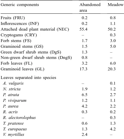
Canopy structure was assessed at the time of the biomass maximum (end of July) by stratified clip-ping (Monsi and Saeki, 1953) of a square plot of 0.3–0.5 m lateral length. Thickness of the harvested layers ranged between 0.02 and 0.04 m. Silhouette area was determined by the means of an area me-ter (LI-3100, Li-Cor, Lincoln, USA). The harvested plant material was separated as follows: leaves were separated into those having the largest fractional con-tribution to total PAI. Eight species were identified at the abandoned area (Nardus stricta, Plantago atrata, Polygonum viviparum, Potentilla aurea, Ranuncu-lus acris, Trifolium pratense, Trollius europaeus, Vaccinium myrtillus) and nine at the meadow (Al-chemilla vulgaris, N. stricta, P. atrata, P. viviparum, P. aurea, R. acris, Rhinanthus alectorolophus,
T. pratense, T. europaeus). In the following the first letter of the generic name followed by the full species names will be used to abbreviate species names, un-less otherwise indicated. The remaining leaves were pooled to three functional groups: forbs, graminoids and dwarf shrubs (FL, GL and DL, respectively). Sep-aration into these functional groups was also made for stems of forbs and graminoids (FS, GS); for dwarf shrubs further distinction was made between green (DgS) and non-green (DngS) woody stems. The re-maining plant components, i.e. fruits (FRU), inflores-cences (INF), attached dead plant material (NEC) and cryptogams (CRY), were pooled over all species. Alto-gether 17 components, as shown in Table 2, were dis-tinguished at each site. In the following, these pooled quantities will be referred to as generic components. Phytoelement inclinations and widths were measured in the field with a hand inclinometer with a 5◦ accu-racy and a ruler, respectively (Tappeiner and Sapinsky, 1999).
Table 2
Species and components (percentage of total PAI) distinguished within the canopies of an abandoned area and a meadow at the study area Monte Bondonea
Generic components Abandoned area
Meadow
Fruits (FRU) 0.2 0.8
Inflorescences (INF) 0.2 1.1
Attached dead plant material (NEC) 55.4 50.2
Cryptogams (CRY) – 0.3
Forb stems (FS) 1.7 3.0
Graminoid stems (GS) 1.5 5.0
Green dwarf shrub stems (DgS) 1.3 – Non-green dwarf shrub stems (DngS) 0.8 –
Forb leaves (FL) 3.2 6.0
Graminoid leaves (GL) 17.3 20.3 Leaves separated into species
A. vulgaris – 0.1
N. stricta 1.9 1.2
P. atrata 6.5 2.7
P. viviparum 1.2 1.1
P. aurea 4.2 2.2
R. acris 0.3 0.2
R. alectorolophus – 0.3
T. pratense 0.6 1.3
T. europaeus 1.3 4.2
V. myrtillus 2.4 –
aAbbreviations for the generic components are given in
2.3. Models
2.3.1. General aspects
In the present study, a one-dimensional, multi-layer model is used to compute the fluxes of CO2, latent and sensible heat between the vegetation and the at-mosphere. It consists of coupled micrometeorological and physiological modules. The micrometeorological modules compute radiative transfer (separately for the PPFD, near-infrared (NIR) and long-wave radiation (IR)) and the attenuation of wind speed. The profiles of CO2, H2O and air temperature within the canopy are not modelled, but instead, either measured values are used as input data or the profiles are kept constant (see below). The environmental variables computed in the micrometeorological modules represent the driving forces for the energy balance model, which partitions absorbed energy into emitted long-wave radiation, latent and sensible heat fluxes. Net photo-synthesis, respiration, and stomatal conductance are calculated in a sub-module of the energy balance, whenever applicable (see below).
The phytoelements making up the canopy are sep-arated into one of three physiological categories: A, B and C. Category A phytoelements are characterised by the ability to assimilate CO2, such as leaves, green stems of herbaceous species and cryptogams. Cate-gory B covers the canopy components characterised by a positive CO2 balance. All phytoelements with a positive CO2 balance, including non-green, but also green woody stems of dwarf shrubs (Siegwolf, 1987), fit into this category. Finally, phytoelements classified as category C do not show any CO2 gas exchange. Attached dead plant material is assigned to the last category, thereby neglecting CO2loss resulting from microbial decay. Besides CO2 gas exchange, the three physiological categories also differ with respect to water vapour exchange: phytoelements classified as category A are capable of losing water via their stomata. Members of categories B and C are assumed to be non-transpiring (Anderson et al., 2000), which neglects peridermal transpiration by woody stems, as well as the loss of water absorbed by dead plant material.
Some of the following theory is kept short on pur-pose, since it was already topic of one of our previous papers, to which we refer for details. Symbols and abbreviations are given in Nomenclature.
2.3.2. Leaf gas exchange
Following theory developed by Farquhar and co-workers (Farquhar, 1979; Farquhar et al., 1980; Farquhar and Von Caemmerer, 1982), later modi-fied according to Harley and Tenhunen (1991), CO2 assimilation is either entirely limited by the kinetic properties of RUBISCO and the respective concen-trations of the competing gases CO2 and O2 at the sites of carboxylation (WC) or by electron transport (WJ), which limits the rate at which RuBP is regener-ated. Limitations of RuBP regeneration arising from the availability of inorganic phosphate for photophos-phorylation are not considered in the present ap-proach. Net photosynthesis A may then be expressed as where Oi and Ci are the concentrations of O2 and CO2 in the intercellular space, respectively, τ is the specificity factor for RUBISCO (Jordan and Ogren, 1984), Rdaythe rate of CO2evolution from processes other than photorespiration and min{ } denotes “the minimum of”.
To be able to predict gas exchange at the leaf level, the photosynthesis model has to be combined with a model predicting stomatal conductance (Harley and Tenhunen, 1991). For this purpose the empirical model by Ball et al. (1987), modified according to Falge et al. (1996), was chosen
gsv =gmin+1000Gfac(A+IfacRdark) hs
Cs, (2)
where gsv is the stomatal conductance, gmin the minimum or residual stomatal conductance and hs and Cs are the relative humidity and the CO2 con-centration at the leaf surface. Gfac is an empirical coefficient representing the composite sensitivity of stomata to these factors. Rdark is the dark respiration and Ifac represents the extent to which dark respi-ration is inhibited in the light. Stomatal opening in response to PPFD is controlled via (A+IfacRdark), which gives an estimation of gross photosynthetic rate and is considered to be related to energy require-ments for maintaining guard cell turgor (Falge et al., 1996).
according to Fick’s law:
Ci=Cs−1600A
gsv
, (3)
where 1600 accounts for the difference in diffusivity between CO2and H2O (Farquhar and Sharkey, 1982) and the difference in the units of A and gsv. Due to the fact that net photosynthesis and stomatal conductance are not independent, the model must solve for Ciin an iterative fashion (Harley and Tenhunen, 1991). Further details on the leaf gas exchange model may be found in Wohlfahrt et al. (1998).
2.3.3. Bole respiration
An Arrhenius-type equation is used to model respi-ration of woody stems as a function of temperature
Rbole=Rbole(Tref)exp
1H
where Rbole(Tref) is the respiration rate at the refer-ence temperature (Tref, 273.16 K), TpK the absolute temperature, R the universal gas constant and1Haan activation energy.
2.3.4. The energy balance
Phytoelement surface temperatures are estimated solving their energy balance equation (Campbell and Norman, 1998) where Rabs is the bi-directional absorbed short-wave and long-wave radiation, Lethe emitted long-wave ra-diation, LE and H represent latent and sensible heat exchange, respectively,εcis the phytoelement thermal emissivity, σ the Stefan–Boltzmann constant,ρ and cpare the density and the specific heat of dry air, re-spectively,γ is the psychrometric constant and gtvthe total conductance to water vapour. The calculation of gtvdepends on whether water is present on the phyto-element surfaces or not. In the absence of surface water, gtvis calculated as
gtv=
gsvgbvδ gsv+gbvδ
, (6)
where gbvis the all-sided boundary layer conductance to water vapour andδis a Boolean variable indicating whether leaves have stomata on one(δ=0.5)or both (δ=1)leaf sides. Leaves and, due to the lack of ap-propriate data, green stems of the investigated species are treated as hypostomatous, although the latter might be supposed to have stomata distributed on the entire surface. Eq. (6) implies no latent heat exchange for dry phytoelements of categories B and C, since for thesegsv = 0. If phytoelements are wet (either due to dew formation, or the interception of precipitation or dew dripping down from upper canopy layers), gtv reduces to gbv (Nikolov et al., 1995). Dew forms on a phytoelement surface if the surface temperature drops below the dew point temperature of the surrounding air (Monteith, 1957). The calculations of dew dynam-ics recognise that phytoelements hold water up to a maximum capacity before the onset of dripping to the canopy components below, following an approach de-scribed by Wilson et al. (1999) and Anderson et al. (2000).
Boundary layer conductances to water vapour are modelled, following Nikolov et al. (1995), as the larger of the conductances resulting from forced and free convective exchange, making use of the non-dimensional groups (e.g. Monteith and Unsworth, 1990; Nobel, 1991). Characteristic phytoelement di-mensions are taken as 0.7 width for leaves and dead attached plant material, approximating these as flat intersecting parabolas, and as the diameter for the remaining canopy components, approximating their shape as cylinders (Campbell and Norman, 1998). In order to account for the enhancement of bound-ary layer conductances due to the turbulent nature of outdoor environments a factor of 1.4 is included (Campbell and Norman, 1998). The boundary layer conductance to water vapour is converted to that for heat by the factor 0.924. The energy balance equation is solved in an analytical fashion following Nikolov et al. (1995), re-arranging it in a quartic form first proposed by Paw U (1987).
2.3.5. Within-canopy profiles of wind speed, CO2 and H2O concentration, and air temperature
which attenuation proceeds exponentially (Wohlfahrt et al., 2000). A simple half-order closure scheme is adopted for the concentration profiles of CO2 and H2O, i.e. they are assumed to be constant within the canopy, which yields only small errors in the com-putation of CO2 and latent heat fluxes (Baldocchi, 1992). Sensible heat exchange, on the other hand, depends strongly on the within-canopy air tempera-ture profile (Baldocchi, 1992), which in the present approach is pre-described using measured profiles of within-canopy air temperature. Continuous profiles are generated by linear interpolation between air tempera-tures measured at different heights (usually seven). In the case that measured profiles of CO2 and H2O are available, the half-order closure assumption is aban-doned and the same procedure as for air temperature is followed.
2.3.6. Radiative transfer
The model of radiative transfer treats the canopy as a horizontally homogeneous, plane-parallel turbid medium in which multiple scattering occurs on the el-ements of turbidity (phytoelel-ements) of the different components, each having their own optical and geo-metrical properties. The canopy is divided into suffi-ciently small, statistically independent layers, within which self-shading may be considered negligible and phytoelements to be distributed symmetrically with respect to the azimuth. Hemispherical reflection and transmission of radiation, which are allowed to be unequal, are assumed to be lambertian. Nine incli-nation classes are considered. Details are given in Appendix A.
2.3.7. Numerical aspects
The present model involves five iteration loops: (i) two nested iterations in the gas exchange module in order to find a combination of A, Ci and gsv, (ii) one iteration in order to find leaf temperatures compat-ible with the long-wave radiation profile (Wohlfahrt et al., 2000), and (iii) one iteration in finding the pro-files of PPFD, NIR and IR. For the latter, a relaxation method, by which the scattered fluxes are added to the fluxes already there, is applied to solve for Eqs. (A.6), (A.9)–(A.13), as described in Goudriaan (1977). The corresponding convergence criteria were chosen as a compromise between numerical accuracy and compu-tation time. For Ci and gsvconvergence criteria were
taken as 1mmol mol−1 and 1 mmol m−2s−1, respec-tively, for leaf temperatures as 0.1◦C, and for radiation as 0.05 W m−2. Tests with more stringent convergence criteria demonstrated that the aforementioned criteria are adequate.
Numerical stability and computation time of the above iterations also depend on their initialisation, i.e. on the choice of the starting values for the variables which are iterated for (except for (iii), where no start-ing values are employed; see above). In the first loop of the first time step, temperatures of sunlit and shaded phytoelements are initialised as air temperature+3◦C and air temperature, respectively, Ci as 0.75Ca (Sage, 1994), and gsv as 500 and 300 mmol m−2s−1 for sunlit and shaded phytoelements of category A, re-spectively. Since the gas exchange module is called every time phytoelement temperatures are up-dated, the values of Ci, gsv, for category A, and equilibrium temperatures calculated during the previous loop are used as starting values in the following loops of the same time step. During subsequent time steps, the final values from the previous time steps are used.
The most time consuming iteration is the one for phytoelement equilibrium temperatures, due to the large number of calculations (including nested iter-ations in gas exchange module) involved. Using the above criteria, phytoelement temperatures usually converge within 3–6 loops. In the model of radiative transfer four loops are usually necessary to reach convergence in the NIR, three for the PPFD and IR. The model thus accounts for fourth-order scattering in the NIR waveband and for third-order scattering in the PPFD and IR wavebands.
2.3.8. Model testing
The model was extensively tested employing a budget approach: energy balance closure (RNveg =
the same absolute temperatures. Under these condi-tions long-wave radiation absorption and emission by phytoelements are equal, and hence RNveg is equal to zero. The discretisation into nine sky sectors gives rise to a small imbalance (Goudriaan, 1977), causing net radiation to deviate from the intended value, this deviation is though less than 0.5%. Consistency of the model of dew dynamics was checked by tracking the fate of water formed on phytoelements as dew. At the end of the simulation run, the total amount of dew formed during the run needs to be equal to the sum of dew evaporated into the atmosphere, dripped down to the soil surface and still present on the phytoelements. Using this approach, no imbalances were found using a wide range of meteorological forcing variables.
Model performance was assessed with respect to both quantitative and qualitative correspondence to measured data (cf. Pachepsky et al., 1996). Pearson’s correlation coefficient and the F-test were used in order to test whether the model is quantitatively ade-quate. Qualitative model performance was evaluated by analysing deviations from 1:1 correspondence in the y-intercept and the slope obtained from lin-ear regression analysis of observed versus predicted values.
3. Results and discussion
3.1. Parameterisation
3.1.1. Gas exchange
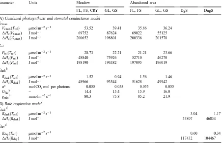
Parameterisation of the leaf gas exchange models of the investigated species was the topic of a previous paper (Wohlfahrt et al., 1998), and will therefore not be repeated. The corresponding parameters are shown in Table 3. The gas exchange parameters for the generic components, though, require some comments: Wohlfahrt et al. (1999) recently presented model parameters for the maximum rate of carboxylation (VCmax) and the potential rate of RuBP regeneration (Pml) for 30 mountain grassland species, from which they derived generic model parameters for forbs, graminoids and dwarf shrubs, separately for mead-ows and abandoned areas. These parameters were adopted for leaves and stems of forbs and graminoids as shown in Table 4. Since V. myrtillus was by far the dominating dwarf shrub on the abandoned area, the
corresponding model parameters from Wohlfahrt et al. (1998) were used, instead of the generic dwarf shrub parameters from Wohlfahrt et al. (1999). Dark respi-ration parameters (unpublished, except for the species from the Monte Bondone study area, cf. Wohlfahrt et al., 1998) for these groups were calculated from the same data set. The apparent quantum yield of net photosynthesis at saturating CO2 concentration, α (Harley and Tenhunen, 1991), was assigned an average value of 0.055 mol CO2mol per photon (Bal-docchi and Meyers, 1998). Parameters of the stomatal conductance model (Gfac and gmin) must be consid-ered site specific (Wohlfahrt et al., 1998) and were hence calculated, separately for the three functional groups, by averaging over the respective species from each site (Table 4).
Parameters describing bole respiration of green and non-green stems of dwarf shrubs were derived from gas exchange measurements on Rhododendron ferrug-ineum by Siegwolf (1987) and converted from a mass to an area basis using data by Gazarini (1988). In his studies Siegwolf (1987) found that respiration rates, in particular those of green stems, differed in light and darkness. This effect is accounted for by using two different parameter sets, both for green and non-green stems, depending on illumination, darkness being de-fined as PPFD<25mmol m−2s−1(Table 4). 3.1.2. Radiative transfer
Table 4
Parameters of (A) the combined photosynthesis and stomatal conductance model for leaves and stems of forbs (FL and FS, respectively), graminoids (GL and GS, respectively) and cryptogams (CRY), and (B) of the bole respiration model for green (DgS) and non-green (DngS) stems of dwarf shrubsa
Parameter Units Meadow Abandoned area
FL, FS, CRY GL, GS FL, FS GL, GS DgS DngS
(A) Combined photosynthesis and stomatal conductance model VCmax
Vcmax(Tref) mmol m−2s−1 53.52 39.41 35.86 36.24
1Ha(VCmax) J mol−1 69752 87624 69022 55125
1Hd(VCmax) J mol−1 200652 198801 200336 201578
Pml
Pml(Tref) mmol m−2s−1 28.73 22.21 21.21 23.66
1Ha(Pml) J mol−1 48840 75926 52710 46270
1Hd(Pml) J mol−1 198190 194482 197095 196019
Rdarkb
Rdark(Tref) mmol m−2s−1 1.52 0.94 1.56 1.46
1Ha(Rdark) J mol−1 48966 93544 51628 49942
αc mol CO
2mol per photons 0.055 0.055 0.055 0.055
Gfacb – 14.4 15.4 15.9 16.0
gminb mmol m−2s−1 80.3 75.8 85.2 21.9
(B) Bole respiration model Rdarkd
Rdark(Tref) mmol m−2s−1 3.04 1.17
1Ha(Rdark) J mol−1 53807 46834
Rdayd
Rday(Tref) mmol m−2s−1 0.60 0.34
1Ha(Rday) J mol−1 117432 104467
aFor abbreviations and symbols, see Nomenclature. 1S(V
Cmax) and 1S(Pml) were fixed for all components of (A) at 656 and
643 J K−1mol−1, respectively (cf. Wohlfahrt et al., 1998). Parameters are from Wohlfahrt et al. (1999), except for Footnotes b–d. bWohlfahrt et al. (unpublished).
cBaldocchi and Meyers (1998). dSiegwolf (1987).
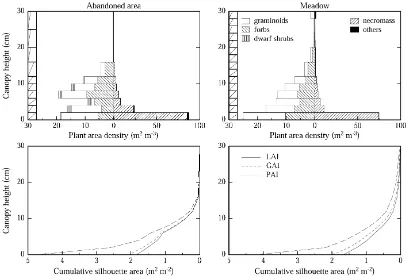
Phytoelement inclination distributions, as well as widths, of the generic components were found as av-erages over the species for which detailed measure-ments were made, weighted by their PAI.
The model of radiative transfer assumes a random distribution of phytoelements (Goudriaan, 1977). Clumping occurs if phytoelements are grouped to-gether, so that more radiation penetrates as compared to a random distribution; the reverse is true for a reg-ular distribution, where phytoelements tend to avoid each other’s presence (Baldocchi and Collineau, 1994). Assuming a random phytoelement distribution in a simpler version of the present model, Wohlfahrt et al. (2000) found reasonable correspondence
be-tween modelled and measured within-canopy profiles of PPFD. Using the present, more elaborate model version together with the same data set as Wohlfahrt et al. (2000), model predictions match observed val-ues even closer (data not shown). The assumption of a random phytoelement distribution is hence kept.
Fig. 1. Vertical canopy structure for an abandoned area and a meadow at the study area Monte Bondone. Photosynthetically active and non-active canopy components are drawn to left and the right of the figures in the upper panel, respectively. Average phytoelement inclination angles are indicated to the left of the figures in the upper panel. The lower panels show the cumulative LAI, green area index (GAI) and PAI.
Table 5
Vegetation and soil optical properties for the wavebands of PPFD, NIR and IR (for abbreviations, see Nomenclature)
PPFD NIR IR reflection
Reflection Transmission Reflection Transmission
FL, FS, GL, Gsa 0.12 0.06 0.38 0.37 0.04b
FRU, INF, CRYa 0.12 0.06 0.38 0.37 0.04b
DL, DgSa 0.09 0.06 0.43 0.39 0.04b
DngSc 0.15 – 0.35 – 0.04b
NECa 0.42 0.13 0.53 0.21 0.04b
Soil 0.15d – 0.25e – 0.07f
reflectance is influenced in a complex fashion by sev-eral factors, such as water content (e.g. Jacquemoud et al., 1992) and soil physical and chemical proper-ties (e.g. Baumgardner et al., 1985). Parameters have been thus chosen such that they fall into the middle of the range described in literature for each of the three wavebands (Table 5).
3.2. Sensitivity analysis
In order to asses potential deviations in model predictions introduced by selecting inappropriate pa-rameter values, a sensitivity analysis was conducted varying, within a reasonable range, the parameters for which no measured values were available. This concerns vegetation and soil optical properties, dwarf shrub bole respiration parameters, and inclination distribution, width and physiology of the generic components. Simulations were conducted for two contrasting weather scenarios, a clear and an over-cast day, respectively, using meteorological forcing variables as they are typically encountered at the study area at the end of July (Table 6). The same meteorological variables were used for both canopies, thus neglecting potential feedback effects by canopy processes on these variables.
3.2.1. Optical properties
Soil and vegetation optical properties determine the amount of absorbed, emitted (long-wave only) and scattered radiation, the latter two being made avail-able for interaction with other objects. Increases in soil reflectance result in radiation formerly absorbed by the soil, i.e. energy “lost” to the vegetation,
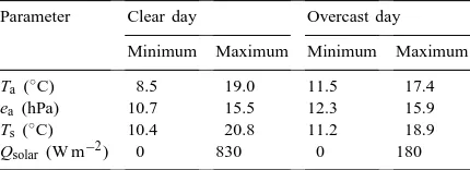
be-Table 6
Meteorological forcing variables employed in sensitivity analysisa
Parameter Clear day Overcast day Minimum Maximum Minimum Maximum Ta(◦C) 8.5 19.0 11.5 17.4
ea (hPa) 10.7 15.5 12.3 15.9
Ts(◦C) 10.4 20.8 11.2 18.9
Qsolar (W m−2) 0 830 0 180 aClear and overcast day scenarios refer to typical weather
situations at the study area during the end of July. CO2
concen-tration and wind speed above the canopy were kept constant at 350mmol mol−1 and 2 m s−1, respectively. For abbreviations, see
Nomenclature.
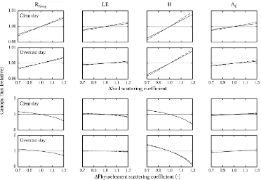
ing redirected into the canopy (Asner and Wessman, 1997). Part of this upward radiation flux is absorbed, increasing RNveg, the vegetation net radiation, which in turn causes phytoelement temperatures to rise as indicated by an increase in H (Fig. 2). Higher leaf temperatures in turn stimulate LE (Fig. 2) by in-creasing the air-to-leaf-vapour-pressure-difference (ALVPD). AC profits from the additional availabil-ity of scattered PPFD. Quantitatively the effects are though almost negligible, being less than 1% for al-terations in soil optical properties of 30% (Fig. 2). Increasing phytoelement scattering coefficients leads to a decrease in radiation absorption at the phytoele-ment level and ultimately to increased radiation loss from the canopy (Asner and Wessman, 1997). The decreased net radiation causes phytoelement temper-atures to decline, as indicated by the decrease of H and LE (Fig. 2). The decrease in LE is though fairly small, due to the fact that decreased leaf temperatures cause ACslightly to increase (Fig. 2), which through Eq. (2) in turn increases gsv and hence ultimately LE. Decreased phytoelement temperatures cause the emission of long-wave radiation by the phytoelements to decrease and hence increase RNveg, this effect is though offset by an increase of the reflected radiation component (Fig. 2). Alterations of the vegetation opti-cal properties are quantitatively much more important as compared to those of the soil, e.g. increasing the phytoelement scattering coefficients by 30% results in a decrease in H by up to 90%. Differences between the abandoned area and the meadow, as well as with regard to clear and overcast weather situations, are generally small, both for soil and vegetation optical properties.
3.2.2. Dwarf shrub bole respiration
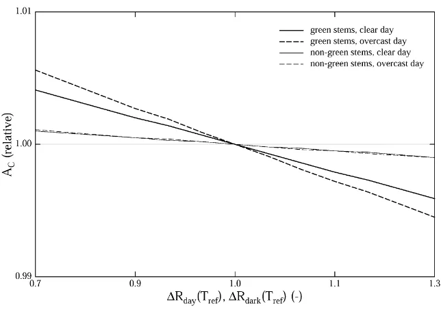
Altering the respiration rate of green and non-green stems of dwarf shrubs affects canopy carbon gain of the abandoned area only slightly, as shown in Fig. 3. This is not surprising, given the small contribution to the total PAI of 2.1% (Table 2).
3.2.3. Structural and functional properties of the generic components
Fig. 2. Sensitivity analysis investigating the effects of altered soil and vegetation optical properties on daily sums (sun rise till sun set) of vegetation net radiation (RNveg), latent (LE) and sensible (H) heat exchange, and canopy net photosynthesis (AC) of an abandoned area
(solid lines) and a meadow (dashed lines) at the study area Monte Bondone. Exchange rates are expressed relative to those obtained using the original parameters. Note the different scales on the y-axis.
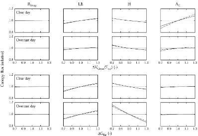
parameters for these components were found by averaging, as described above and in Wohlfahrt et al. (1999). The sensitivity of bulk canopy exchange rates to these parameters was assessed as shown in Fig. 4. The photosynthetic potential was altered by varying the maximum rate of carboxylation (VCmax), and by scaling the potential rate of RuBP regeneration (Pml) and the dark respiration rate (Rdark) in proportion to VCmax. According to the model of Wohlfahrt et al. (1998) this procedure is equivalent to altering the ni-trogen content. Increasing VCmax leads to an increase in AC, accompanied by an increase in LE due to the dependence of gsvon A as expressed in Eq. (2). Since no additional energy is available to the system, RNveg is virtually constant and H decreases accordingly. Stomatal conductance was altered by varying Gfac, a coefficient which determines the correlation between net photosynthesis and stomatal conductance (Ball et al., 1987). Increasing Gfac leads to an increase of gsvand hence LE, which, in terms of available energy,
is compensated by a decrease in H. Higher stomatal conductances allow for more CO2to enter the leaves, increasing Ci and in turn AC. Differences between clear and overcast day scenarios are generally small, effects being slightly more pronounced during clear days. Carbon gain of the meadow is slightly more sensitive to alterations of photosynthetic parameters as compared to the abandoned area (Fig. 4). This is mainly due to the fact that at the meadow the generic components make up a larger portion of the total biomass as compared to the abandoned area. In fact, if put to a PAI basis, it turns out that the generic components of the abandoned area would be more efficient in using additional photosynthetic potential.
Fig. 3. Sensitivity analysis investigating the effects of altered respiration rates of green and non-green dwarf shrub stems on the daily sum (sun rise till sun set) of canopy net photosynthesis (AC) of an abandoned area at the study area Monte Bondone. Exchange rates are
expressed relative to those obtained using the original parameters.
effect) sensitivity for phytoelement widths (data not shown).
3.3. Validation
The ability of the multi-component vegetation– atmosphere-transfer (VAT) model to adequately sim-ulate the exchange of CO2 and energy between the vegetation and the atmosphere is assessed by compar-ing model predictions with independent above-canopy measurements of CO2and energy exchange.
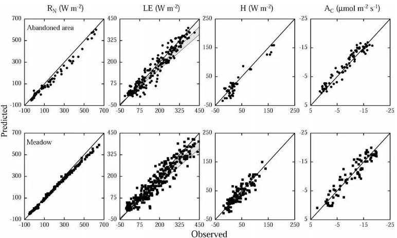
The net radiation balance of the canopy (RN) must be simulated accurately, if we are to compute realistic latent and sensible heat and CO2 flux densities (Baldocchi and Harley, 1995). A comparison between observed and predicted net radiation flux densities (Fig. 5) reveals, that the model is fairly well capa-ble of simulating low values of RN, but increasingly underestimates high values, as also indicated by the linear regression analysis in Table 7. During clear days around noon, the upwelling radiation flux den-sity is overestimated by up to 60 W m−2, which is about twice the value quoted as the typical accuracy of net radiation measurements (Halldin and
Fig. 4. Sensitivity analysis investigating the effects of altered leaf gas exchange model parameters of the generic groups on the daily sums (sun rise till sun set) of vegetation net radiation (RNveg), latent (LE) and sensible (H) heat exchange, and canopy net photosynthesis (AC)
of an abandoned area (solid lines) and a meadow (dashed lines) at the study area Monte Bondone. Exchange rates are expressed relative to those obtained using the original parameters.
accounted for. For forest ecosystems it should, how-ever, be noted, that the upwelling radiation may show considerable spatial variation due to the heterogeneity of the underlying soil–vegetation surface. Droppo and Hamilton (1973) report a 13% difference in net radi-ation above a deciduous forest when measured simul-taneously from towers 15 m apart, and Anthoni et al. (1999) found upwelling radiation to vary spatially by 60 W m−2 above an open-canopied ponderosa pine forest. For the grasslands under study the spatial variation in RN remains yet to be determined. We conclude that a combination of the effects of the het-erogeneity of the underlying soil–vegetation surface, measurement accuracy, and a small systematic over-estimation of phytoelement temperatures is likely to be the main reason for the observed underestimation of RN.
Validating canopy latent and sensible heat exchange proves somewhat problematic, since the
Fig. 5. Comparison of observed versus predicted values of net radiation (RN), latent (LE) and sensible (H) heat exchange, and canopy net
photosynthesis (AC) of an abandoned area and a meadow at the study area Monte Bondone. Solid lines indicate 1:1 correspondence. The
two lines below the 1:1 line on the LE plot indicate estimated 1:1 correspondence for pure canopy evapotranspiration, assuming a 10 and 20% reduction by soil evaporation (Rutter, 1979).
water vapour released by soil and vegetation (Finnigan and Raupach, 1987). Using water vapour pressures from above the canopy thus artificially increases the ALVPD, and ultimately transpiration (given stomatal conductance remains constant). The resulting error in the computation of whole canopy LE may though
Table 7
Results of a linear regression analysis of observed versus predicted values of net radiation (RN) and the fluxes of latent (LE) and sensible
(H) heat, as well as net photosynthesis (AC)a
Parameter Site Slope y-Intercept r F Fcrit.
RN A 0.94±0.02 −19.75±4.04 0.99 3409.12 7.04
M 0.92±0.01 −0.58±1.24 0.99 46826.80 6.84
LE A 0.95±0.02 1.18±3.77 0.96 2576.90 6.76
M 0.89±0.02 8.52±3.49 0.95 2817.87 6.72
H A 0.92±0.05 −3.08±2.73 0.95 387.88 7.22
M 0.90±0.04 3.09±2.08 0.89 496.46 6.84
AC A 0.94±0.03 1.20±0.29 0.97 1070.57 6.96
M 0.96±0.04 0.26±0.50 0.94 569.96 6.96
aModel performance is evaluated by the slope and the y-intercept of a regression line through observed versus predicted values (mean±standard error), Pearson’s correlation coefficient (r) and by comparison of the F-value (F) with the critical F-value (Fcrit., F-value
atp=0.01) (A: abandoned area, M: meadow).
and direction of the soil sensible heat flux are fairly variable (e.g. Raupach et al., 1997). Its sign depends on whether soil surface temperatures are above or below that of the adjacent air layer, whereas soil evaporation remains positive even if soil surface tem-peratures are below air temperature as long as the water vapour gradient is positive (Campbell, 1985). Soil surface temperatures (data not shown) are gener-ally above that of the adjacent air layer at the meadow (a positive sensible heat flux), whereas a distinct diur-nal pattern is observed at the abandoned area. There, the soil surface, as compared to the adjacent air layer, heats up more quickly during the morning, the soil sensible heat flux being positive until the early after-noon, when soil surface temperature drops below air temperature, the sensible heat flux then being negative until the morning. The model thus should underesti-mate measured H at the meadow, whereas both over-and underestimation should occur at the abover-andoned area. Yet, as shown in Table 7, H is slightly underes-timated at both sites. Since H is fairly sensitive to the profile of within-canopy air temperature (Baldocchi, 1992), this discrepancy may be due to errors associ-ated with unattended measurements of within-canopy air temperatures, which are somewhat tricky in such dense canopies. Plant parts moved by the wind easily displace the thermocouples from the intended posi-tions exposing them to solar radiation or causing con-tact with neighbouring canopy elements or supporting experimental structures. Clearly, further experiments, aiming at separating vegetation and soil energy fluxes, are needed to satisfactorily validate the present model. As shown in Fig. 5, the model is well capable of predicting canopy net photosynthesis, the slopes and y-intercepts being close to 1 and 0, respectively, as well as the F-values exceeding the critical ones (Table 7). At the abandoned area, though, the residuals indi-cate a slight qualitative deficiency, a larger fraction of measured values being overestimated (Fig. 5). This is likely to be caused by the spatial heterogeneity within the fetch of the BREB measuring system. Parts of the abandoned area are composed by stands dominated by dwarf shrubs (mainly V. myrtillus), which are charac-terised by smaller carbon gains as compared to the investigated canopy. This is due to their smaller leaf photosynthetic potential (Cernusca et al., 1992; Bahn et al., 1999; Wohlfahrt et al., 1999), as well as their un-favourable ratio between photosynthetically active and
non-active biomass (Tappeiner and Cernusca, 1996, 1998; see also Fig. 1 and Tables 1 and 2). During pe-riods when the wind conveys air parcels originating from dwarf shrub dominated parts of the abandoned area past the sensors of the measuring system, overes-timation by the model occurs. Similar problems have been encountered in several other modelling studies (e.g. Williams et al., 1996). These data could be re-moved from the validation data set by excluding the sectors where such contamination is likely to occur, this was though not done in the present case, given the minor nature of the resulting deviations.
3.4. Model application
In the present approach, modelling is taken to a very detailed level, explicitly considering the different structural and functional characteristics of the various vegetation components. The price for this high level of detail, inevitably, is a large number of input pa-rameters, which clearly represents a drawback for ap-plication of the present modelling approach at larger spatial and/or temporal scales for which such detailed data will hardly be available (Running et al., 1999). In the following, we hence employ the present model in order to test for the quantitative effects of some sim-plifying assumptions, which may need to be made if one aims at predictions at larger spatial and/or tempo-ral scales.
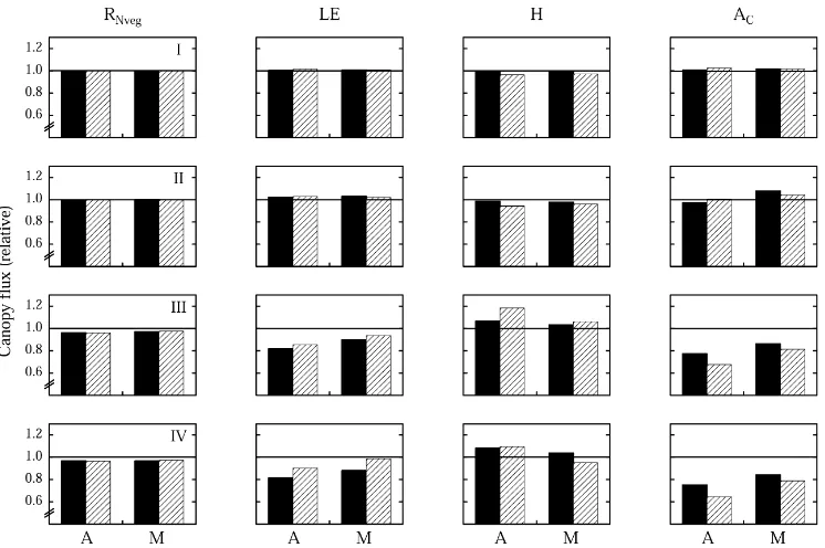
Fig. 6. Sensitivity analysis investigating the effects of assuming (I) a spherical phytoelement angle distribution, (II) species physiology to be represented by three functional groups, and a homogeneous vertical phytoelement distribution in the canopy as a whole (III) and separately in an upper and lower layer (IV), on vegetation net radiation (RNveg), latent (LE) and sensible (H) heat exchange, and canopy
net photosynthesis (AC) for an abandoned area (A) and a meadow (M) at the study area Monte Bondone. Daily sums (sun rise till sun set)
of exchange rates are expressed relative to those obtained using the original parameters. Black bars indicate clear, hatched bars overcast weather conditions.
fluxes — the former because of the small amount of phytoelement area (Fig. 1), the latter because of the prevailing unfavourable environmental conditions, mainly the reduced light availability.
When dealing with the gas exchange of multi-species vegetation communities some simplifications regard-ing the description of leaf physiology need to be made. Up to this point we followed a mixed ap-proach, using species-specific parameters for the key-species, whereas the remaining species were cat-egorised into three functional groups and assigned respective generic values (see above). In the follow-ing the concept of functional groups (cf. Dawson and Chapin, 1993; Chapin, 1993) will be extended to the photosynthetically active phytoelements of all species, i.e. with regard to leaf gas exchange only forbs, graminoids and dwarf shrubs will be distin-guished (for parameters refer to Table 4). As shown in Fig. 6–II, such a reduction of physiological input
parameters, keeping all other parameters constant, affects bulk canopy processes by less than 6%. This example clearly shows the potential of using the con-cept of functional groups for aggregating leaf physi-ological parameters, given of course a representative data basis exists. Recently, much effort in compiling corresponding data sets has been undertaken (e.g. Wullschleger, 1993; Reich et al., 1998a,b; Niinemets, 1999; Medlyn et al., 1999; Wohlfahrt et al., 1999), so that similar approaches should become feasible in the near future also for other ecosystems.
in Fig. 6–IV, we hence assumed the total PAI, but not the vertical distribution of phytoelements, to be avail-able as input data. In a second scenario (Fig. 6–III), which aims at capturing the obvious bi-layered struc-ture of many mountain grasslands (e.g. Tappeiner and Cernusca, 1994), we further divided this single vegetation layer into two separate ones, within which phytoelements were again assumed to be distributed in a homogeneous manner. For this purpose the same heights as used for the model of wind speed (Table 1; Wohlfahrt et al., 2000) were adopted to separate the upper from the lower canopy layer. As can be seen from Fig. 6–III and IV, both simplifications produce considerable deviations in the resulting predictions, in particular for LE, H and AC which are altered by up to 35%, indicating the importance of accounting for the vertical phytoelement distribution in heteroge-neous (mountain grassland) canopies (Raupach and Finnigan, 1988; Tappeiner and Cernusca, 1998).
4. Conclusion
A model is presented which allows for simulating vegetation–atmosphere CO2 and energy exchange of multi-component, multi-species grassland canopies, explicitly taking into account the structural and func-tional properties of the various components and species. For parameterisation a mixed approach is followed, using species-specific parameters for the components with the largest fractional contribution to the total biomass, and generic, average values for the remainder. The performance of the model in compar-ison with field measurements is broadly satisfactory, although validation of sensible and latent heat fluxes suffers from the difficulty to discern between the con-tributions from the soil and the vegetation. A sensitiv-ity analysis reveals that the model is fairly sensitive to vegetation optical properties, indicating the need for own measurements, which were not available in the present study. The model was found to be less sensitive to soil optical properties, phytoelement in-clination distributions and widths of the generic com-ponents, as well as bole respiration parameters. The latter finding though probably needs to be reconciled, if dwarf shrub dominated canopies are to be investi-gated. Using generic physiological parameters for the three main functional groups (forbs, graminoids and
dwarf shrubs), proved to produce acceptable results, despite a high sensitivity of the model to these param-eters. This shows the potential of using the concept of functional groups for aggregating leaf physiological parameters, given a representative data basis exists. If predictions of bulk canopy exchange rates are of sole interest, assumption of a uniform spherical phytoelement angle distribution appears sufficient. Though, due to the distinct vertical heterogeneity of the investigated canopies considerable deviations in predicted bulk exchange rates are observed, if a ver-tical homogeneous distribution of phytoelements is assumed. Future model developments should aim at including the soil compartment (soil surface energy balance, soil water and heat transport, soil respi-ration), which would also ease model validation. Furthermore, it seems desirable to include turbu-lent transport of momentum, air temperature, water vapour and CO2 concentration within and above the canopy.
Acknowledgements
This work was conducted within the EU-TERI-project ECOMONT (EU-TERI-project No. ENV4-CT95-0179, framework IV of EU) and the FWF-project P13963-BIO (Austrian National Science Foundation). We would like to express our gratitude to Jan Goudri-aan for inspiring discussions on the model of radia-tive transfer, Ingrid Horak for her assistance during eco-physiological field work, and Sigrid Sapinsky and Christian Newesely for operating and maintaining the micrometeorological measurements. The Centro di Ecologia Alpina and the Servizio Parchi e Foreste Demaniali (both Trento/Italy) are gratefully acknowl-edged for their logistic support.
Appendix A. Model of radiative transfer
and Collineau, 1994)
where G is the projection of the phytoelements in-clined at an angleλinto the directionβ(De Wit, 1965; Ross, 1981; Goudriaan, 1977), and may be calculated as
Because of the non-linear response of photosynthe-sis to PPFD the radiation incident on shaded and sunlit canopy areas must be considered separately. Shaded phytoelements receive diffuse light only, while sunlit ones receive both diffuse and direct radiation, the lat-ter incident at an angleβ∗, the elevation of the sun. The attenuation of beam radiation (Qdir) is calculated as
where np stands for the number of phytoelements. The fraction of sunlit phytoelement area, fsl, is proportional to the attenuation of direct radiation and hence given by
fsl(j )=
Qdir(j+1)
Qdir(n+1) (A.5)
forQdir(n+1) >0, otherwisefsl(j )=0. The flux of diffuse radiation in the canopy consists of diffuse ra-diation from the atmosphere and of diffused, scattered beam radiation. For the treatment of diffuse radiation, the upper and lower hemispheres viewed by the phy-toelements are divided into nine sectors of 10◦each (due to this discretisation sinβ in Eq. (A.1) needs to be replaced by 12[sin(10β)+sin(10(β−1))] if nine sectors are distinguished; Jan Goudriaan, personal
communication). The downward short-wave fluxes (Qd) within the canopy consist of the non-intercepted radiation from above (first part on the right-hand side of Eq. (A.6)), the diffuse radiation transmitted from above and reflected from below downwards (second part on the right-hand side of Eq. (A.6)), and the direct radiation transmitted in the down-ward direction (third part on the right-hand side of Eq. (A.6)) as
The prime (β′) denotes that the angle refers to scat-tered radiation,ρcandτcare phytoelement reflection and transmission coefficients, respectively, and ξ is a reflection–transmission distribution function as de-fined by Goudriaan (1977). The scattered, i.e. reflected and transmitted, radiation, as well as emitted radia-tion, is distributed as
Bl(p, j, β′)=
Bu(β′)Pi(p, j, β′)
P9
β=1Bu(β)Pi(p, j, β)
, (A.7)
where Bu is the zonal distribution of radiation scat-tered by a lambertian reflector (Goudriaan, 1977), cal-culated for nine sky sectors as (Jan Goudriaan, per-sonal communication)
be-low and reflected from above upwards, and the direct radiation reflected in the upward direction as
Qu(j, β) When calculating the within-canopy profile of long-wave radiation it has to be accounted for that the phytoelements themselves emit long-wave radia-tion. Since leaves do not transmit long-wave radiation (τc = 0), the calculation of the downward and up-ward fluxes is considerably simpler as compared to Eqs. (A.6) and (A.9), i.e.
The downward (Eq. (A.10)) and upward (Eq. (A.11)) fluxes of long-wave radiation thus consist of the non-intercepted flux from above and below, respec-tively, the upward radiation reflected downwards and the downward radiation reflected upwards, re-spectively, and the emitted radiation. The latter is calculated as the weighted mean flux from sunlit and shaded phytoelements, which radiate at ab-solute temperatures TpKsl and TpKsh, respectively, using the Stefan–Boltzman law. Emissivity εc is assumed to be equal to (1 − ρc) (Kirchhoff’s law).
At the soil surface, the lower boundary condition of the model, light is reflected/emitted lambertian as
Qu(0, β)=ρsBu(β′) 9
X
β=1
Qd(1, β)
for short-wave radiation, (A.12)
Lu(0, β)=Bu(β)
for long-wave radiation, (A.13)
whereρs is the wavelength-dependent soil reflection coefficient and TsKthe absolute soil surface tempera-ture.
The soil and the sky emitted long-wave radiation, as well as the short-wave radiation, represent state variables, the corresponding radiation fields are hence calculated only once per time step. Whereas the long-wave radiation emitted by the phytoelements de-pends upon their temperatures and in turn influences their temperatures via the energy balance (Eq. (5)), making it necessary to solve in an iterative fashion for their equilibrium temperatures.
Now that the within-canopy radiation field has been specified, it is possible to calculate the amount of radiation intercepted and/or absorbed by the various canopy components. Short-wave radiation incident on shaded phytoelements is calculated as
and the radiation incident on sunlit phytoelements is
where Qdir(n +1) stands for the direct radiation measured on a horizontal plane above the canopy. Long-wave radiation is distributed equally among sunlit and shaded canopy components as
L(p, j )=
The results of Eqs. (A.14) and (A.15) may be used di-rectly to calculate assimilation, since PPFD in the leaf gas exchange model (Eq. (6) in Wohlfahrt et al., 1998) refers to an incident light basis. In order to calculate absorbed short-wave and long-wave radiation, as it is required for the leaf energy balance (Eq. (5)), Qshade, Qsunand L need to be multiplied by an absorption co-efficient, which is calculated as(1−(ρc+τc)).
Solar geometry, determining the position of the sun in the sky, is calculated using the equations given in Campbell and Norman (1998). Total solar radiation, as well as the partitioning of solar radiation into di-rect and diffuse, PPFD and NIR components, is either modelled using the approach described in Goudriaan (1977) and Goudriaan and Van Laar (1994), or mea-sured values (as described in the previous section) are used instead. Similarly, sky long-wave radiation may be either estimated using the equations by Brutsaert (1984) and Monteith and Unsworth (1990), or mea-sured values be used. The corresponding algorithms have been presented in Wohlfahrt et al. (2000).
References
Anderson, M.C., Norman, J.M., Meyers, T.P., Diak, G.R., 2000. An analytical model for estimating canopy transpiration and carbon assimilation fluxes based on canopy light-use efficiency. Agric. For. Meteorol. 101, 265–289.
Anthoni, P.M., Law, B.E., Unsworth, M.H., 1999. Carbon and water vapor exchange of an open-canopied ponderosa pine ecosystem. Agric. For. Meteorol. 95, 151–168.
Asner, G.P., Wessman, C.A., 1997. Scaling PAR absorption from the leaf to landscape level in spatially heterogeneous ecosystems. Ecol. Model. 103, 81–97.
Asner, G.P., Wessman, C.A., Schimel, D.S., Archer, S., 1998a. Variability in leaf and litter optical properties: implications for BRDF model inversions using AVHRR, MODIS, and MISR. Remote Sens. Environ. 63, 243–257.
Asner, G.P., Wessman, C.A., Archer, S., 1998b. Scale dependence of absorption of photosynthetically active radiation in terrestrial ecosystems. Ecol. Appl. 8, 1003–1021.
Bahn, M., Cernusca, A., Tappeiner, U., Tasser, E., 1994. Wachstum krautiger Arten auf einer Mähwiese und einer Almbrache. Ver. Ges. Ökol. 23, 23–30.
Bahn, M., Wohlfahrt, G., Haubner, E., Horak, I., Michaeler, W., Rottmar, K., Tappeiner, U., Cernusca, A., 1999. Leaf photosynthesis, nitrogen contents and specific leaf area of grassland species in mountain ecosystems under different land use. In: Cernusca, A., Tappeiner, U., Bayfield, N. (Eds.), Land-use Changes in European Mountain Ecosystems. ECOMONT — Concepts and Results. Blackwell Wissenschafts-Verlag, Berlin, pp. 247–255.
Baldocchi, D.D., 1992. A Lagrangian random walk model for simulating water vapor, CO2 and sensible heat flux densities
and scalar profiles over and within a soybean canopy. Boundary Layer Meteorol. 61, 113–144.
Baldocchi, D.D., 1993. Scaling water vapor and carbon dioxide exchange from leaves to canopy: rules and tools. In: Ehleringer, J.R., Field, C.B. (Eds.), Scaling Physiological Processes: Leaf to Globe. Academic Press, San Diego, CA, pp. 77–116. Baldocchi, D.D., Collineau, S., 1994. The physical nature of
solar radiation in heterogeneous canopies: spatial and temporal attributes. In: Caldwell, M.M., Pearcy, R.W. (Eds.), Exploitation of Environmental Heterogeneity by Plants. Academic Press, San Diego, CA, pp. 21–71.
Baldocchi, D.D., Harley, P.C., 1995. Scaling carbon dioxide and water vapor exchange from leaf to canopy in a deciduous forest. II. Model testing and application. Plant Cell Environ. 18, 1157– 1173.
Baldocchi, D.D., Meyers, T., 1998. On using eco-physiological, micrometeorological and biogeochemical theory to evaluate carbon dioxide, water vapor and trace gas fluxes over vegetation: a perspective. Agric. For. Meteorol. 90, 1–25.
Ball, J.T., Woodrow, I.E., Berry, J.A., 1987. A model predicting stomatal conductance and its contribution to the control of photosynthesis under different environmental conditions. In: Biggens, J. (Ed.), Progress in Photosynthesis Research, Vol. IV. Proceedings of the VII International Congress on Photosynthesis. Martinus Nijhoff, Dordrecht, pp. 221–224. Baumgardner, M.F., Silva, L.F., Biehl, L.L., Stoner, E.R., 1985.
Reflectance properties of soils. Adv. Agron. 38, 1–44. Berry, J.A., Collatz, G.J., Denning, A.S., Colello, G.D., Fu, W.,