PROCESSING LIDAR WAVEFORM DATA FOR 3D VISUAL ASSESSMENT OF
FOREST ENVIRONMENTS
F. Pirotti a,b,* , A. Guarnieri b, A. Masiero b, A. Vettore b , E. Lingua a
a Department of Land, Environment, Agriculture and Forestry, University of Padova Italy
b CIRGEO Interdepartmental Research Center of Geomatics, University of Padova, Italy- (francesco.pirotti, emanuele.lingua, alberto.guarnieri, andrea.masiero, antonio.vettore)@unipd.it
Commission V/WG3
KEY WORDS: Forestry, Full Waveform Lidar, 3D modelling, Visual representation
ABSTRACT:
The objective of this report is to present and discuss a work-flow for extracting, from full-waveform (FW) lidar data, formats which are compatible with common information systems (GIS) and statistical software packages. Full-waveform, specifically for forestry, got attention from the scientific community because a more in-depth analysis can add valuable information for classification and modelling of related variables (e.g. biomass). In order to assess if this is feasible and if the results are useful, the end-user has to deal with raw datasets from lidar sensors. In this study case we propose and test a work-flow which is implemented through a self-developed software integrating ad-hoc C++ libraries and a graphical user interface for an easier approach by end-users. This software allows the user to add raw FW data and produce several products which can successively be easily imported in GIS or statistical software. To achieve this we used some state-of-the-art methods which have been extensively reported in literature and we discuss results and future developments. Results show that this software package can effectively work as a tool for linking raw FW data with forest-related spatial processing by providing punctual information directly derived from the FW data or area-based aggregated information for a more generalized description of the earth surface.
1. INTRODUCTION
Lidar sensors have developed towards being faster and more accurate. Online processing of the return laser signal returns data as discrete points in space (i.e. point clouds) with attributes like energy (i.e. intensity) and echo ordinal position. In the last ten years there has been increased interest into analysis of the whole return signal, referred to as full-waveform (FW). This is recorded by a digitizer which samples at defined time intervals (usually ~1 ns) the amount of incoming energy. This implies an increase in the amount of data which has to be stocked in memory, moved between PCs and processed to extract significant information for end users. At least ten times more space is required for this type of data, as well as exponentially more cpu-time depending on adopted approaches for processing the FW data.
Numerous related investigations argue pros and cons of using FW (Ussyshkin and Theriault, 2011), but all agree that FW brings potential improvements related to two aspects: (i) enhancement of detection weak return echoes, which results in an increase in overall point density (Toth et al., 2011) in some cases by a factor of x2 (Reitberger et al., 2008) and (ii) the availability of metrics extracted from the distribution of Ei = f(ti) in the FW, e.g., amplitude, echo width, backscatter cross-section, backscatter cross-section per illuminated area and backscatter coefficient, and (iii) the user has greater control over data interpretation (Mallet and Bretar, 2009) and more information can be extracted.
In particular forests present a peculiar type of target for laser beams, as the tree structure presents multiple small targets, represented by leaves and branches, and structurally different
canopies return different waveforms responses, thus land-cover classification can be improved (Neuenschwander et al., 2009). The focus of this paper is to present a workflow for processing lidar full-waveform data and convert extracted information in different representations and formats which allow further processing with conventional geographic information systems and statistical analysis tools. The presentation is divided in the following sections: (i) an overview of FW lidar applications in forestry, with a brief analysis of existing approaches for information extraction, (ii) a description of the test dataset used and the study area, (iii) an explanation of chosen methods and the processing steps in the work-flow, (iv) a discussion on resulting products and future improvements.
1.1 Full waveform lidar in forestry
Literature has widely investigated lidar applications for extracting vegetation information, especially for the field of forestry (Hyyppä et al., 2012). Forestry gets a particular advantage from lidar data, compared to data from other active or passive remote sensors, because the receiver can record multiple returns from a single emitted laser pulse, thus multiple targets along its path, which cause only partial obstruction, are detected, if not too close to each (Mallet and Bretar, 2009). This also allows the pulse to have a high probability of reaching the ground plane which is a critical aspect of for a relatively accurate estimation of the ground plane (F. Pirotti et al., 2013a). Tree canopies have characteristic texture with gaps which allow the laser beam to reach the ground surface (Lefsky et al., 2002). Information on echoes from the ground and from the canopy
allow to model crowns and estimate number of stems and tree heights with sufficient accuracy to be used for inventorial purposes, depending on canopy closure and tree structure (Alberti et al., 2013; Pirotti, 2011). In several forest types and conditions, the estimation of biomass in a stand has been proven to give important results, due to the capability for prediction of lidar-derived stand height or mean height of dominant and co-dominant trees (Hall et al., 2005; Lefsky et al., 1999; Means, 1999). In this context FW lidar adds the possibility of an analysis of the return signal to further analyze forest cover. The objective can be the classification of forest land-cover and species (Neuenschwander, 2009) or more forest-related parameters like biomass (Alexander et al., 2010; Baccini et al., 2012; Koch, 2010) or for inventory purposes (Anderson et al., 2008).
2. MATERIALS AND METHODS
2.1 Study area
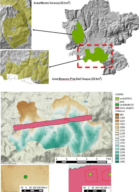
The area used for testing the method is located in the northern part of the Italian peninsula, in the area of Asiago. This area is one of many which make up a collection of test sites for the NEWFOR project (NEW technologies for a better mountain FORest timber mobilization) in the Alpine Space Programme, a broader investigation which will see four distinct study sites relative to the Italian partners, providing different forest scenarios, i.e. even-aged high-forest, multi-layered high-forest and coppice, sampled with circular areas of 20 m radius stratified by forest structure categories.
Figure 1. (top) the Asiago region with the two study areas; (bottom) the Boscon area with the analysed strip and the plots.
All areas have been surveyed with airborne lidar campaigns. In our specific case the survey was done with Optech ALTM GEMINI 1064 nm wavelength, 167 kHz max pulse repetition frequency (PRF), 0.25 mrad (1/e) beam divergence, along with the Optech waveform digitizer (8-bit amplitude resolution, 1 ns sample rate, 70 kHz max acquisition rate), operated in June 2012. Figure 1 shows the specific location of a sub-area which was used for testing, the Boscon area.
2.2 Calibration procedures
Calibration over vegetated areas poses a challenge as the structure of canopy and stem presents multiple and non-homogeneous surfaces which are intercepted by the laser beam along its path. As the recorded waveform P(t) is a result of the emitted waveform T(t) convoluted with response from different sources as in equation below (Jutzi and Stilla, 2006a, 2006b)
P(t) = T(t)*S(t)*M(t)*P(t)+N(t) (1)
where S(t) is the surface response, M(t) is the response of the measuring unit, P(t) is the spatial beam distribution, and N(t) is the background noise. In our case M(t) is considered negligible and P(t) is considered constant and not a Gaussian distribution for the reasons reported in (Adams et al., 2012, p. 687) and also empirically assessed in an investigation by the author which is not yet published.
The above assumption leaves us with two components, noise and surface response. The latter is influenced by the following aspects: (a) spherical loss, (b) topographic and (c) atmospheric effects (Höfle and Pfeifer, 2007). The first two are related to the targets and are very complex to model, whereas the latter is a degradation of the energy content of the laser beam as it travels through the atmosphere due to physical laws of absorption and reflection by gas particles and is an easier problem.
A common approach is to simply correct recorded energy (En) with a range-squared relationship using a standard range (Rs) and the pulse range (Rn) as shown below.
�= ��
2
��2 (2)
Because of the complexity of the physical interactions and also the complexity of the forest surface, in our work-flow the processing for calibration is done with an empirical mathematical model. The function parameters in the model are estimated using targets which have the same cross-section and which are surveyed at different ranges, e.g. the asphalt runway of the airport used for take-off and landing of the vehicle like in (Coren and Sterzai, 2006) and reported in (Höfle and Pfeifer, 2007). This allows creating a look-up-table (LUT) for direct correction of the return energy. Our study area is over forests and the topic of investigation is uniquely focused on vegetation, therefore we assume that targets will be smaller than the size of the laser footprint and the target scattering area relevant for explaining FW metrics (i.e cross-section σ [m2]) remains the same independent of the size of the laser footprint area: i.e. as long as the target is small compared to the footprint (Wagner, 2010). Empirical correction is important to allow the creation of comparable products between sample areas extracted from different strips in different flying missions of a FW survey (F. Pirotti et al., 2013b).
2.3 Waveform analysis
In our case the digital representation of the waveform consist, for each emitted pulse, in one or more segments with an arrow of n 8-bit integers representing incoming energy level in a 1 ns interval. The segment represents what the digitizer buffer saves in memory when the sensor detects a significant return echo (above background noise level). To describe the waveform two main steps are necessary: the first step is to detect peaks, i.e. echoes from reflective targets, and the second step is to define metrics related to the peak which describe the cross-section of the surface which caused the corresponding echo.
2.3.1 Peak detection: in literature there are a vast number of investigations over approaches for discriminating peaks from the FW signal. Faster methods are the thresholding of local maxima (Billauer, 2008) and zero crossing of first derivative (Toth et al., 2011). Other methods based on spline-fitting (Roncat et al., 2011) or Gaussian decomposition (Mallet and Bretar, 2009) have proven to give higher peak detection rate, i.e. x1.2 – x2, but are require higher costs in terms of execution time i.e. x14 - x3000 (Toth et al., 2011).
We applied the thresholding technique in this implementation of the method, removing any signal which was not above the noise level as shown in Figure 2. Noise was calculated by taking several samples of digitizer segments without echoes as calculating the mean energy level and the standard deviation (σ). The energy baseline was defined as any signal below the mean + 3σ level (Figure 2). No noise-removal process was applied it takes computation time and requires the correct definition of smoothing parameters which might become a source of error in the process.
A peak is defined as local maxima, a value which is higher than its neighbours around it. So a window has to define the neighbour domain. In our case the window consists in the number of time bins (ns) where we consider equal to the maximum width where a local maximum can be mistaken as a peak due to noise. The following conditions have to be met for the signal at time t to be defined as a peak:
{ �
> �+ …� � � > �− …�
(3)
Where E(t) is the energy count at time t which is being tested for peak condition, i is the window width in time bins defining the neighbourhood.
2.3.2 Waveform fitting: this process defines the boundaries of the signal which belong to a certain reflective surfaces. An ideal approach is Gaussian decomposition of the signal around the peak assuming that the FW is a sum of Gaussian, like it is for most cases (Mallet and Bretar, 2009) and then define width as full-width-at-half-maximum (FWHM) with the relationship with the standard deviation σ of such function. Many approaches have been tested successfully, see (Stilla and Jutzi, 2009).
Because forest surfaces lead to complex responses and thus complex return signals, we adopted a simpler approach and we define the FWHM as:
� = { �− = 0.5 ∗ �
0 ℎ ��
� = { �+ = 0.5 ∗ �
0 ℎ ��
� + � = ��
(4)
where lw and rw are respectively left width and right width and m is the distance from the time t of peak Et where signal energy falls below half the peak energy (above the energy baseline i.e. noise).
2.3.3 Waveform metrics: this process extracts metrics which characterize the shape of the FW related to the extracted peak. The usual metrics extracted are amplitude i.e. energy of peak corrected with energy baseline and empirically with range/atmosphere, and width as seen in the previous section (FWHM). In our process we also extract the following other metrics: (i) left and right energy, as the integral of energy around the peak see Figure 2 (ii) rise time and fall time as in (Drake et al., 2002) and FW center of mass as the distance to median energy (similal to the HOME metric by same authors).
= ∫�� (5)
Where LE is the left energy relative to peak n (Figure 2) and t1 and t2 are the time bins corresponding to the lw and rw respectively as described in the previous section.
Figure 2. Plot of energy digitizer values over time for a return FW signal: characterization of waveform by amplitude (PE) and partial integral of parts including two echoes.
2.3.4 Data products: the software we present outputs FW metrics in different formats and using different spatial criteria. The first spatial criteria is to extract all data, thus if exporting a strip all data will be written. It has been tested and disk space and memory requirements limit this type of output. The other criteria is to use shapefiles that delimit sample plots to spatially clip data at first step of echo definition, and thus proceed with the FW and metric extraction only on echoes falling inside the sample plots. Sample plots can be points or polygons. In the first case the user has to provide a radius for defining the plot area. A unique textual identifier, defined in a specific attribute column, is required for associating the echoes with sample area. Inside each sample area echoes and respective metrics are kept in tabular format which is then also represented as a point cloud. Another product is created by the spatial aggregation of the metrics using regular gridded formats both in 3D (voxels) and 2D (pixels). In the latter case conventional raster formats are used, where in the former VTK file format is used. In the next page we present results and discuss potential utilizations.
3. RESULTS
3.1 Products
The results from running the process over the data are saved in the following formats (see Figure 3):
(i) VTK formats (Kitware, 2014)
(a) voxel representation (i.e. structured grid) with the medians of each metrics represented as scalars in each cell;
(b) point representation (i.e. unstructured grid) with scalars for each point with metrics’ values;
(ii) several raster representations in GeoTiff format each holding a characteristic defined in the pixel area by four bands for median, standard deviation, 5%, and 95% quantile values of the metric. Minimum and maximum values are not used because they are too much influenced by outliers;
(iii) a textual representation of echoes inside the sample area as table in comma separated value (CSV) format with each column holding the value of the metric for that peak.
Each file created as output is named after the FW file which was used and the shapefile which holds the sample plots’ locations.
Figure 3. From top to bottom: VTK representation, raster grid representation and CSV representation of metrics extracted from the FW.
These files can then be imported respectively in software which allows importing VTK files (e.g. GRASS, Paraview), in conventional GIS software for the GeoTiff raster output, and statistical analysis tools for the CSV files (e.g. R software for statistical computing). These formats can be joined with information from the sample plots which contain ground-truth data (e.g. basal area, diameter at breast height etc…) and models can be tested for correlation.
3.2 Further processing scenarios
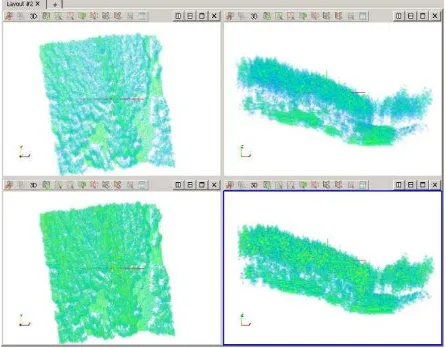
An example of further processing of data extracted from this work-flow is to use the CSV representation for importing in software supporting spatial statistical analysis such as R-cran (R Development Core Team, 2014). Joining FW data extracted with our method from sample plots with ground-truth data surveyed from the plots themselves is the first step towards modelling, e.g. with regression techniques. In Figure 4 a sample plot with a point cloud derived from our method had a ground surface defined via an iterative morphological approach (F. Pirotti et al., 2013c; Francesco Pirotti et al., 2013) which allows to then proceed into defining a canopy height model (CHM) and regression analysis to define biomass (Vaglio Laurin et al., 2014) or tree detection (Pirotti, 2010).
Figure 4. (top-left) level-plot of ground plane raster before filter and (top-right) after filter; (bottom) representation of fitted ground plane and lidar echoes in the sample area, colour scale represents height from ground plane.
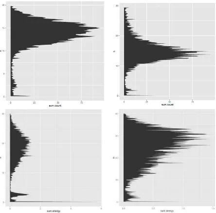
In forestry this is a fundamental step as an accurate ground surface is the first step towards defining vertical characteristics of the vegetation which are in turn correlated to biodiversity and to the dynamics of tree growth. Figure 5 shows results of aggregating data by plots and by vertical bins of 0.15 cm (corresponding to 1 ns two-way travel time of laser pulse); specifically the number of peaks falling in the vertical slice are reported. Plots have a circular shape and have a 20 m radius.
Figure 5. Profiles showing the vertical distribution FW peaks in four different plots.
4. DISCUSSION AND CONCLUSIONS
In this paper we presented results of processing FW data for extracting products for further processing of data for forest applications. We also show a scenario for further processing such formats for initial statistical analysis. This is an important step for connecting research and development to end-users which are used to handling more conventional data formats. Data analysts use geographic data and geographic information systems and statistical analysis tools and can take advantage of such tool. More complex interactions with existing datasets related to land management, e.g. biodiversity (Piragnolo et al., 2014), or even collaborative portals (Pirotti et al., 2011) which integrate FW data with other remote sensing data can bring added value to end users. Having a lot of data does not imply having a lot of information, especially if users cannot extract important components from such data. That is the reason that exporting data representations of the FW information can bring help in that direction.
The methods used have been chosen for speed over accuracy, and a future development ideally would allow the user to choose which method to use for peak extraction and waveform characterization. This would allow more room for specific processing according to the study area, which might have different types of land cover – high or low vegetation – or different forest structure – coppice or high-forest – or also different canopy density thus requiring a more time-consuming peak detection algorithm for detecting peaks in weak echoes below the initial canopy layers. Geometric and radiometric correlations also have to be studied in order to provide other methods other than an empirical range/atmosphere correction, especially in case no clean targets are available for creating a LUT. Being FW a very promising source of data for forest applications, efforts in this directions will provide useful tools for researchers and data analysts.
ACKNOWLEDGEMENTS
This work has been done as part of the NEWFOR project (NEW technologies for a better mountain FORest timber mobilization) in the Alpine Space Programme (2-3-2 FR).
REFERENCES
Adams, T., Beets, P., Parrish, C., 2012. Extracting More Data from LiDAR in Forested Areas by Analyzing Waveform Shape. Remote Sensing, 4, 682–702. doi:10.3390/rs4030682
Alberti, G., Boscutti, F., Pirotti, F., Bertacco, C., De Simon, G., Sigura, M., Cazorzi, F., Bonfanti, P., 2013. A LiDAR-based approach for a multi-purpose characterization of Alpine forests: an Italian case study. iForest - Biogeosciences and Forestry, 6, 156–168. doi:10.3832/ifor0876-006
Alexander, C., Tansey, K., Kaduk, J., Holland, D., Tate, N.J., 2010. Backscatter coefficient as an attribute for the classification of full-waveform airborne laser scanning data in urban areas. ISPRS Journal of Photogrammetry and Remote Sensing, 65, 423–432. doi:10.1016/j.isprsjprs.2010.05.002
Anderson, J., Plourde, L., Martin, M., Braswel, B., Smith, M., Dubaya, R., Hofton, M., Blair, J., 2008. Integrating waveform lidar with hyperspectral imagery for inventory of a northern temperate forest. Remote Sensing of Environment, 112, 1856– 1870. doi:10.1016/j.rse.2007.09.009
Baccini, A., Goetz, S.J., Walker, W.S., Laporte, N.T., Sun, M., Sulla-Menashe, D., Hackler, J., Beck, P.S.A., Dubayah, R., Friedl, M.A., Samanta, S., Houghton, R.A., 2012. Estimated carbon dioxide emissions from tropical deforestation improved by carbon-density maps. Nature Climate Change, 2, 182–185. scanning. International Journal of Remote Sensing, 27, 3097– 3104. doi:10.1080/01431160500217277
Drake, J.B., Dubayah, R.O., Clark, D.B., Knox, R.G., Blair, J.B., Hofton, M.A., Chazdon, R.L., Weishampel, J.F., Prince, S., 2002. Estimation of tropical forest structural characteristics using large-footprint lidar. Remote Sensing of Environment, 79, 305–319. doi:10.1016/S0034-4257(01)00281-4
Hall, S.A., Burke, I.C., Box, D.O., Kaufmann, M.R., Stoker, J.M., 2005. Estimating stand structure using discrete-return lidar: an example from low density, fire prone ponderosa pine forests. Forest Ecology and Management, 208, 189–209. doi:10.1016/j.foreco.2004.12.001
Höfle, B., Pfeifer, N., 2007. Correction of laser scanning intensity data: Data and model-driven approaches. ISPRS Journal of Photogrammetry and Remote Sensing, 62, 415–433. doi:10.1016/j.isprsjprs.2007.05.008
Hyyppä, J., Holopainen, M., Olsson, H., 2012. Laser Scanning in Forests. Remote Sensing, 4, 2919–2922. doi:10.3390/rs4102919
Jutzi, B., Stilla, U., 2006a. Range determination with waveform recording laser systems using a Wiener Filter. ISPRS Journal of Photogrammetry and Remote Sensing, 61, 95–107. doi:10.1016/j.isprsjprs.2006.09.001
Jutzi, B., Stilla, U., 2006b. Characteristics of the measurement unit of a full-waveform laser system. Revue Française de Photogrammétrie et de Télédétection, 182, 17–22.
Kitware, I., 2014. File Formats for VTK [WWW Document].
The VTK User’s Guide,. URL
http://www.vtk.org/VTK/img/file-formats.pdf
Koch, B., 2010. Status and future of laser scanning, synthetic aperture radar and hyperspectral remote sensing data for forest biomass assessment. ISPRS Journal of Photogrammetry and
Remote Sensing, 65, 581–590.
doi:10.1016/j.isprsjprs.2010.09.001
Lefsky, M.A., Cohen, W.B., Acker, S.A., Parker, G.G., Spies, T.A., Harding, D., 1999. Lidar Remote Sensing of the Canopy Structure and Biophysical Properties of Douglas-Fir Western Hemlock Forests. Remote Sensing of Environment, 70, 339– 361. doi:10.1016/S0034-4257(99)00052-8
Lefsky, M.A., Cohen, W.B., Parker, G.G., Harding, D.J., 2002. Lidar Remote Sensing for Ecosystem Studies. BioScience, 52, 19. doi:10.1641/0006-3568(2002)052[0019:LRSFES]2.0.CO;2
Mallet, C., Bretar, F., 2009. Full-waveform topographic lidar: State-of-the-art. ISPRS Journal of Photogrammetry and Remote Sensing, 64, 1–16. doi:10.1016/j.isprsjprs.2008.09.007
Means, J., 1999. Use of Large-Footprint Scanning Airborne Lidar To Estimate Forest Stand Characteristics in the Western Cascades of Oregon. Remote Sensing of Environment, 67, 298– 308. doi:10.1016/S0034-4257(98)00091-1
Neuenschwander, A.L., 2009. Landcover classification of small-footprint, full-waveform lidar data. Journal of Applied Remote Sensing, 3, 033544. doi:10.1117/1.3229944 Impact on Biodiversity. ISPRS International Journal of Geo-Information, 3, 599–618. doi:10.3390/ijgi3020599
Pirotti, F., 2010. Assessing a Template Matching Approach for Tree Height and Position Extraction from Lidar-Derived Canopy Height Models of Pinus Pinaster Stands. Forests,. doi:10.3390/f1040194
Pirotti, F., 2011. Analysis of full-waveform LiDAR data for forestry applications: a review of investigations and methods. iForest - Biogeosciences and Forestry,. doi:10.3832/ifor0562-004
Pirotti, F., Guarnieri, A., Vettore, A., 2011. Collaborative Web-GIS Design: A Case Study for Road Risk Analysis and Monitoring. Transactions in GIS, 15, 213–226. doi:10.1111/j.1467-9671.2011.01248.x
Pirotti, F., Guarnieri, A., Vettore, A., 2013a. State of the Art of Ground and Aerial Laser Scanning Technologies for High-Resolution Topography of the Earth Surface. European Journal of Remote Sensing, 46, 66–78. doi:doi: 10.5721/EuJRS20134605
Pirotti, F., Guarnieri, A., Vettore, A., 2013b. Analysis of correlation between full-waveform metrics, scan geometry and land-cover: an application over forests. ISPRS Annals of Photogrammetry, Remote Sensing and Spatial Information Sciences, II-5/W2, 235–240. doi:10.5194/isprsannals-II-5-W2-235-2013
Pirotti, F., Guarnieri, A., Vettore, A., 2013c. Vegetation filtering of waveform terrestrial laser scanner data for DTM production. Applied Geomatics, 5, 311–322. doi:10.1007/s12518-013-0119-3
Pirotti, F., Guarnieri, A., Vettore, A., 2013. Ground filtering and vegetation mapping using multi-return terrestrial laser scanning. ISPRS Journal of Photogrammetry and Remote Sensing, 76, 56–63.
R Development Core Team, 2014. The R Manual [WWW Document]. URL http://www.r-project.org/
Reitberger, J., Krzystek, P., Stilla, U., 2008. Analysis of full waveform LIDAR data for the classification of deciduous and coniferous trees. International Journal of Remote Sensing, 29, 1407–1431. doi:10.1080/01431160701736448
Roncat, A., Bergauer, G., Pfeifer, N., 2011. -spline deconvolution for differential target cross-section determination in full-waveform laser scanning data. ISPRS Journal of Photogrammetry and Remote Sensing, 66, 418–428. doi:10.1016/j.isprsjprs.2011.02.002
Stilla, U., Jutzi, B., 2009. Waveform Analysis for Small-Footprint Pulsed Laser Systems, in: Shan, J., Toth, C.K. (Eds.), Topographic Laser Ranging and Scanning: Principles and Processing. CRC Press, pp. 215–234.
Toth, C., Laky, S., Zaletnyik, P., Grejner-Brzezinska, D., 2011. Peak detection from full-waveform data, in: International LiDAR Mapping Forum. New Orleans.
Ussyshkin, V., Theriault, L., 2011. Airborne Lidar: Advances in Discrete Return Technology for 3D Vegetation Mapping. Remote Sensing, 3, 416–434. doi:10.3390/rs3030416
Vaglio Laurin, G., Chen, Q., Lindsell, J.A., Coomes, D.A., Frate, F. Del, Guerriero, L., Pirotti, F., Valentini, R., 2014. Above ground biomass estimation in an African tropical forest with lidar and hyperspectral data. ISPRS Journal of Photogrammetry and Remote Sensing, 89, 49–58. doi:10.1016/j.isprsjprs.2014.01.001
Wagner, W., 2010. Radiometric calibration of small-footprint full-waveform airborne laser scanner measurements: Basic physical concepts. ISPRS Journal of Photogrammetry and
Remote Sensing, 65, 505–513.
doi:10.1016/j.isprsjprs.2010.06.007