DETECTION OF SINGLE TREE STEMS IN FORESTED AREAS FROM HIGH DENSITY
ALS POINT CLOUDS USING 3D SHAPE DESCRIPTORS
N. Amiria,b∗, P. Polewskia, W. Yaoa, P. Krzysteka, A. K. Skidmoreb
aDepartment of Geoinformatics, Munich University of Applied Sciences, Munich, Germany - (n.amiri, przemyslaw.polewski,
wei.yao, peter.krzystek)@hm.edu
b Department of Natural Resources, Faculty of Geo-Information Science and Earth Observation (ITC), University of Twente,
Enschede, The Netherlands - (n.amiri, a.k.skidmore)@utwente.nl
Commission II, WG II/3
KEY WORDS:High density ALS, 3D point clouds, Tree trunk, Classification, Forestry
ABSTRACT:
Airborne Laser Scanning (ALS) is a widespread method for forest mapping and management purposes. While common ALS techniques provide valuable information about the forest canopy and intermediate layers, the point density near the ground may be poor due to dense overstory conditions. The current study highlights a new method for detecting stems of single trees in 3D point clouds obtained from high density ALS with a density of 300 points/m2. Compared to standard ALS data, due to lower flight height (150-200 m) this elevated point density leads to more laser reflections from tree stems. In this work, we propose a three-tiered method which works on the point, segment and object levels. First, for each point we calculate the likelihood that it belongs to a tree stem, derived from the radiometric and geometric features of its neighboring points. In the next step, we construct short stem segments based on high-probability stem points, and classify the segments by considering the distribution of points around them as well as their spatial orientation, which encodes the prior knowledge that trees are mainly vertically aligned due to gravity. Finally, we apply hierarchical clustering on the positively classified segments to obtain point sets corresponding to single stems, and performℓ1-based orthogonal distance regression to robustly fit lines through each stem point set. Theℓ1-based method is less sensitive to outliers compared to the
least square approaches. From the fitted lines, the planimetric tree positions can then be derived. Experiments were performed on two plots from the Hochficht forest in Ober¨osterreich region located in Austria. We marked a total of 196 reference stems in the point clouds of both plots by visual interpretation. The evaluation of the automatically detected stems showed a classification precision of 0.86 and 0.85, respectively for Plot 1 and 2, with recall values of 0.7 and 0.67.
1. INTRODUCTION
Accurate measurements of forest structure are increasingly quired across large areas to support a wide range of activities re-lated to sustainable forest management. Cost-effective and more automated methods are needed to provide tree attribute data for forest ecosystem services. Therefore, remote sensing tools are in-creasingly being used to survey forest structures. However, the spatial extent and spatial resolution of a given sensor are inversely related.
Airborne Laser Scanning (ALS) has become a key tool for gath-ering information on 3D structure of forests (Wulder et al., 2012). The derived information from ALS data can grant de-tailed estimations of forest characteristics and single tree anal-ysis (Yao et al., 2012; Maltamo et al., 2012). Previous studies are showed several properties of single trees such as species, height and crown properties which can be measured with high resolution ALS data (Maltamo et al., 2012). However, limited persistence has been done on the stem detection of single trees. For instance, single tree stems have been determined from the interpolated CHM (Canopy Height Model) at the highest positions(Solberg et al., 2006) or by using hierarchical clustering for stem reflec-tions and reconstrucreflec-tions with a RANSAC-based adjustment (Re-itberger et al., 2007). Due to the low point density and lack of information about the reflection characteristics, minor focus has been given to tree reconstruction using laser hits on the stems (Reitberger et al., 2007; Polewski et al., 2016). In order to detect
∗Corresponding author
stem of trees, data with greater precision would be required to allow a more accurate representation of the actual discontinuities in the single trees (Vauhkonen, 2010).
could estimate tree stem positions with an average proportion of 87%. Wang et al. (2016) performed in the first step, RANSAC based circle fitting of projected stem points, which is later fol-lowed by RANSAC cylinder fitting in 3D space. Polewski et al. (2017) proposed a statistical framework for detecting cylinders based on accumulation and voting in parameter space. The size of the accumulation cell is determined automatically using band-width selection methods for kernel density estimators, which re-laxes the requirement of setting this critical parameter manually or through trial-and-error. The method is applied on a dense 3D point cloud for mapping fallen tree stems. Based on the men-tioned studies, the main advantage of TLS data lies in its capacity to scan a sample plot in forest horizontally and vertically in de-tail. However, important factors such as the occlusion effect and relatively high cost of the instrument transportation from site to site are negatively effecting the use of TLS data. Moreover, the coregistration of several scans covering a study area is an essen-tial step in the interpretation of multi-scan data acquisition. The fully automated registration between several scans at the point level is still challenging.
In standard operational applications of ALS, the flight heights are usually between 400 to 800 m, resulting in point densities up to 30 points/m2. However, an alternative scenario is also possi-ble, where the flying altitude is significantly decreased to below 150 m, for example using a helicopter mounted system or even a UAV with around 50 m flight height. This can be seen as a mid-dle ground between standard ALS and TLS techniques, trading off large area coverage for increased point density. This tradeoff is due to the lower flight altitudes associated with this technique compared to standard ALS campaigns, which results in smaller footprints. Razak et al. (2011) used high resolution DEMs (Dig-ital Elevation Models) extracted from high density ALS data to semi-automatical recognition of morphometric landslide features even under forest canopy. H¨ofle et al. (2012) provided an exam-ple of high density ALS data potential to use for urban vegeta-tion detecvegeta-tion purposes. They used a high point density of 50 points/m2. Khosravipour et al. (2014) also presented an algorithm which is able to create a pit-free CHM raster using full waveform ALS data with 160 points/m2density. The algorithm significantly improves the accuracy of tree detection compared to local max-ima based methods. The data collected by high density ALS sys-tems is less precise in comparison with TLS. However, within an equal time frame, the area that can be investigated by utiliz-ing high resolution ALS is significantly larger than the area in-vestigated with TLS. Also the aforementioned TLS based meth-ods for stem detection are not practical for the applications us-ing ALS data, since the curvature shape of the tree trunk in ALS point clouds is not captured as detailed as in case of TLS. On the other hand, the increased point density, resulting from lower flight height can provide more details in the point clouds compared to standard ALS, enabling the use of 3D spatial descriptors to lo-cate individual tree stems. Therefore, an automated method for stem mapping within high-density ALS data is interesting from forestry application point of view.
The objectives of this study are to develop a new method for sin-gle tree stem detection based on high density ALS data using (i) point and object part level 3D shape descriptors, and (ii)ℓ1 regu-larized line fitting with a prior on orientation. A further objective is (iii) to assess the accuracy of detected tree stems. This paper is motivated by the successful application of high density ALS systems for precise monitoring of vegetation and forest structure, reported in the aforementioned studies. Also, detected tree stems could be used to improve the 3D segmentation algorithm as prior knowledge in terms of the detection rate and the position of trees.
The remainder of this work is structured as follows: Section 2 fo-cuses on the details of our approach. Section 3 shows the exper-iment results. Finally, the results are discussed with conclusions in Sections 4 and 5.
2. METHOD
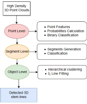
We adapt the method of Polewski et al. (2015) which is origi-nally designed for fallen tree segmentation, to detect the stand-ing stems of sstand-ingle trees from unstructured high density ALS point clouds. The main goal is to detect linear structures in the ALS 3D point clouds which are likely to represent single tree stems. The output of our method is a set of 3D lines which corre-spond to detected stems. The pipeline describing our approach is presented in Fig. 1. Our approach is a three-tiered detection pro-cedure at (i) point, (ii) segment and (iii) object levels. The seg-ment term refers to the grouping of points within a fixed length cylindrical neighborhood which are likely to represent part of a tree stem. Objects refer to entire tree stems which are composed from groups of similarly aligned segments. The method proceeds as follows. First the likelihood of points belonging to a tree stem is estimated. Second, the segments containing the highest proba-bility stem points are detected in the 3D point clouds. Finally the segments are merged through hierarchical clustering to produce single tree stems. In the following, we explain the steps of our method in detail.
Figure 1. Overview of stem detection pipeline.
2.1 Point level
In the input data depending on the forest characteristics, differ-ent objects are presdiffer-ent such as ground vegetation, regenerations, standing tree stems etc. The focus of this step is to obtain for ev-ery point, an estimate of the probability that it belongs to a tree stem. High density ALS data can provide a range of features re-lated mainly to the 3D structure of single trees. The features de-rived from 3D point clouds can be grouped into three categories:
2. Covariance features:set of features derived from eigenval-ues of local neighborhood covariance matrix around target point (see Weinmann et al. (2015)).
3. Normalized height:the relative point heights over the Digi-tal Terrain Model (DTM).
For the point classification level we chose Random Forest (Breiman, 2001) as a binary classifier due to its robust ability to estimate the class probability.
2.2 Segment level
This level focuses initially on generating segment candidates. For each point with high probability, a cylindrical neighborhood with constant radiusrsegand heightlsegis defined. Afterwards, all the points inside the cylinder space are taken into account to perform the least-squares Orthogonal Distance Regression (ODR) (Al-Subaihi and Watson, 2004).This is done by eigenanalysis of the point coordinates’ covariance matrix: the ODR line’s direction is the eigenvector corresponding to the maximum eigenvalue, and this line passes through the points’ centroid. The ODR line be-comes the segment’s axis.
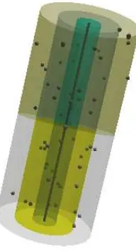
We classify the candidate segments generated in the previous step into the ’positive’ and ’negative’ groups. The ’positive’ group represents the segments which are really parts of tree stems, and the ’negative’ contains branches, ground vegetation, and etc. The first set of segment features are derived from a modified ver-sion of Cylindrical 3d Shape Context (CSC) built around the seg-ments’ axes (Polewski et al., 2015) (see Fig. 2). A spatial distri-bution histogram of points within the cylindrical volume around the segment axis can then be constructed. The point counts inside the histogram bins form the features for the classification.
Figure 2. Cylindrical 3D Shape Context around a segment.
The second set of features are calculated based on the angular deviation of the segment axes from the worldZ. The segments with the deviation larger thanθthr are rejected without regard to remaining feature values. Additionally, the point probability statistics are extracted as another group of features for classifi-cation. In the current study, we looked at the points inside the segment neighborhood and we created the stem point probability histograms quantized at 0.2 intervals, resulting in 5 features.
2.3 Object level
The goal of current level is to take the stem segments with high probability from the previous step and merge them to reconstruct individual tree stems. This is based on the collinearity and mutual distances between segments.
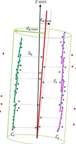
2.3.1 Hierarchical clustering In the next step of the pipeline, the representative ’positive’ segments are merged together. For this purpose, first we have a combination of two distances to cal-culate. The aggregate distancedbetween segmentsSiandSjis the weighted sum of angular deviationdAand the spatial distance between point centroidsdC(see Eq. 1).
d(Si, Sj) =dA(Si, ~~ Sj) +w1.dC( ¯Si,Sj¯) (1)
In the Eq. 1,S~refers to the axis andS¯indicates the point centroid of each segment.w1is the weight component for the spatial dis-tancedC. Fig. 3 shows the angular deviationdA and the spatial distancedCbetween two segments surrounded by cylinders.
Figure 3. The aggregate distancedbetween two segments; the angular deviationdAis shown with green arrow and the spatial
distance between point centroidsdCwith red arrow.
The following hierarchical clustering scheme (Van Der Heijden et al., 2005) is applied to merge ’positive’ segments based on the aggregate distance matrixdexplained above.
1. Assign each point to its own cluster.
2. Find the closest pair of clusters which do not trigger the stopping criterion and merge them into one. The number of clusters reduces by one.
3. Compute the distanceDbetween the new cluster and each of the old clusters.
4. Repeat steps 2 and 3 until no more clusters can be merged under the stopping criterion.
In the current clustering process the distance D between two clusters Ci and Cj is defined as the largest distance d from any combination of member segments. The stopping criterion consists of two conditions. First, when considering two clusters
Ci, Cjif the spatial distancedC between any pair of segments
Sk∈Ci, Sl∈Cjis bigger than a predefined thresholddC,max
then the merging ofCiandCjis aborted. On the other hand, the ODR line is fitted to the set of points belonging to segments in
terminates the merging for that cluster pair. Fig. 4 represents the stopping criterion in the hierarchical clustering phase between segments.
Figure 4. The stopping criterion for clustering the segments. The green lines represent the segments in clusterCiand the magenta lines show the segments in clusterCj, respectively. The red line is the line fitted to both clusters’ points. The red points outside
the cylinder have projected distance greater thandp,max.
2.3.2 Stem line fitting In the final step, for each cluster ex-tracted from the merging step, containing all the stem points, we execute the line fitting procedure. For the fitting, we apply or-thogonal distance regression with theℓ1norm of residuals as the error criterion and a prior on the line’s verticality. The problem is formulated in terms of an energy minimization. The total energy for a lineL,Etot(L)is presented in the Eq. 2. The total energy
Etothas 2 components, the data goodness-of-fit termEd(Eq. 3) and the angular prior termEa(Eq. 4). Theαelement refers to the balance coefficient between energy terms. The angular prior was considered due to the prior knowledge that the tree stems grow almost always vertically. Furthermore, theℓ1norm is a more ro-bust estimator and less sensitive to outliers available in the data compared to theℓ2norm (Al-Subaihi and Watson, 2004). In our
experiment, theℓ2 norm in the segment level and theℓ1 norm is used in the object level, respectively. This decision is related to the computational expenses of theℓ1andℓ2 fittings. Usually,
the number of the segments to process is several orders of mag-nitude higher compared to the stems obtained from hierarchical clustering. On the other hand, theℓ1version is much more com-putationally expensive than theℓ2based method, which makes it intractable to apply for all segments.
Etot(L) =Ed(L) +αEa (2) cluster. Furthermore,Z element in the Eq. 4 representsZ axis of world coordinate system.L(P)term is the projection of point
P onto lineLandwindicatesL’s direction vector. The lineL
is parametrized using 4 valuesa = [a1, ..., a4](Al-Subaihi and Watson, 2004) showed in the Eq. 5:
L(a, t) =
where tis the location parameter. Note that thez component ofwis always positive with a value of 1, and therefore the an-gle between the worldZ axis andwalways lies in the interval [0;π
2]. This allows us to drop the absolute value on the angular
prior termEasince thearccosineis guaranteed to be positive in the mentioned interval.
For the optimization of the orthogonal distance fitting, a two-step method similar to Liu and Wang (2008) as well as Watson (2002) is used. The first step for the re-parametrization computes the pro-jection of all fitted pointsPjonto the current lineL(a, t)to min-imize the distance fromPitoL:
min
tj
kL(a, tj)−Pjk, j= 1, ..., n (6)
The line positionstjcorresponding to the orthogonal projection ontoLcan be recovered using Eq. 7, wherep0= [a1, a3,0]:
tj=(Pj−p0).w
w.w (7)
In the second step, we minimize the energy similar toEtot, but with the projected line positions fixed at{tj}, with respect to shape parameters only, i.e.:
For minimizing the objective (Eq. 8) the BFGS quasi-Newton method is applied (Wright and Nocedal, 1999). The derivative of the energy’s data term with respect to any parameterakis ex-pressed as follows (rj=Pj−L(a, tj)is thej−thresidual):
By splitting the computation into two steps and fixing thetj val-ues, the problem is considerably simplified, because otherwise the termstjin Eq. 9 would depend onak, leading to the necessity of calculating the derivative of the product∂[tj(a)·w(a)]/∂a. Therefore, the derivatives with respect to the entire parameter vector are:
As for the angular deviation termEa, only the axis parameters
a1, a3have a non-zero derivative, given by:
∇a1,a3Ea(a) =
per-form multiple restarts of the optimization with randomly initial-ized starting line hypotheses, and pick the lowest-energy solu-tion. This yields the final fitted lines representing the detected single tree stems for all clusters.
3. EXPERIMENTS
3.1 Materials
Experiments were conducted in the Hochficht forest close to Holzschlag in Ober¨osterreich region which is located in Aus-tria. The study area is a type of mountainous forest with a high structural complexity, dominated by Norway spruce (Picea abies), European beech (Fagus sylvatica) and Silver fir (Abies alba). Two sample plots with the approximate area size of 6844.7 m2
and 17907 m2
and a mean tree density of 272 trees/ha were selected in the mixed forest to construct the experiment. The high density ALS data was acquired in leaf-on condition by the FMM GmbH Company with the VUX-1 scanner integrated in the VP-1 pod in September 20VP-15 with an average point density of 300 points/m2
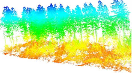
. We assumed that the data is given in a georeferenced coordinate system. The flying altitude between 150-200 m re-sulted in an average footprint size of 88 mm. Fig. 5 shows a sam-ple scene in the 3D point clouds associated with the visible single tree stems.
Figure 5. A point cloud visualization of sample forest scene with multiple visible stems (point clouds of scene colored by height
over DTM).
3.2 Training classifier
We used parts of test plots and two additional plots to train the classifier in the point and segment levels. In the available 3D point clouds, a significant percentage of the stems is not at all represented (specially for the deciduous trees). For every single tree with visible stem, the points and segments were manually marked and assigned either the stem or the non-stem class by visual interpretation, resulting in training sets for binary classifi-cation. The total number of the marked points and segments were 20000 and 564, respectively. This represented about 28% of the total number of the stem points and about 3% of the generated segments in plots 1 and 2.
3.3 Reference data
The schematic class labels which groups individual segments into tree stems were later obtained based on the relative segment posi-tions and orientaposi-tions using visualization. In some cases a single
tree stem was represented in the point cloud, but it was missing from the reference data, due to the lack of evidence in the 3D point clouds. The total number of the labeled stems were 196.
3.4 Choice of parameters
The various control parameter values that we used in our experi-ment for each level is summarized in the Tabel1. The values were assigned experimentally based on the forest characteristics.
Parameters symbols values
Cylinder radius rseg 0.5 m
Cylinder length lseg 2.0 m
Angular deviation θthr 30◦
Spatial distance weight w1 10
Maximum spatial distance dC,max 0.6 m Maximum projected distance dp,max 0.6 m Maximum angular deviation dA,max 20◦ Balance coefficient of energy terms α 0.1×np
Table 1. Control parameters for the single tree stem detection method;nprefers to the number of points inside the clusters.
3.5 Evaluation
In the current experiment we use the ”recall” and ”precision” measures to characterize the detection performance between de-tected and reference tree stems. The ”recall” is defined as the ratio of the reference stem numbers which have at least one associated detected stems to the total number of reference stems. The ”preci-sion” expresses the count of detected stems that were successfully connected to reference stems as a fraction of the total number of detected tree stems. We considered the detected and reference stems as matched if the average projected distance between them was not more than 30 cm. This value was derived based on the maximum DBH of trees in the target area.
4. RESULTS AND DISCUSSION
The procedure for stem detection was applied to the both plots. The output of the single tree stem detection consists of a number of point sets which correspond to the individual stems. The method takes the advantage of the increased point density, which makes more laser reflections available underneath the canopy for regions of test plots dominated by conifers, due to the smaller footprint size compared to the standard ALS. In contrast, the deciduous tree stems are missing in the point clouds due to the dense canopy cover in leaf-on state, and no benefit was achieved despite the lower footprint size. In case that only sparse understory is below the tree base height, stem points are success-fully detected by the expressed classifier training and stem line fitting method.
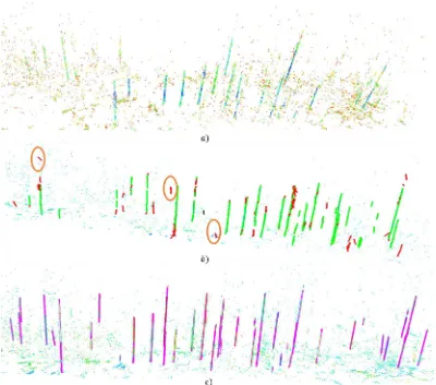
Fig. 6 shows the stem detection results for a sample plot (mixed with deciduous and coniferous trees) in three main levels of point, segment and object. The sample plot contains deciduous and coniferous trees. In Fig. 6a the classification results at the point level based on the high and low point probability on the tree stems are presented. The ”positive” and ”negative” groups of seg-ments are classified using shape context, angular deviation from the worldZand point probability statistics in the Fig. 6b. Finally, at the object level stems with the fitted ODR line (orthogonal dis-tance regression with theℓ1norm) after merging are indicated in
Figure 6. The detection results for a sample plot:(a), (b) and (c) correspond to point, segment and object levels, respectively (see Sections 2.1-2.3). At point level in (a), the red color shows low and blue high probability. The solid green bars in (b) indicate tree stems classified as positive and red bars refer to unmatched tree stems with references. The points which do not belong to the detected stems are removed from analysis and colored as cyan. Orange ellipses outline examples of the false alarms. The fitted magenta lines in
(c) represent the reference tree stems which overlap with colored detected stems (ODR with theℓ1norm).
the analysis.
The detection performance of the proposed method is presented by Fig. 7. Note that in the current test plots, due to the point den-sity and forest characteristics (particularly deciduous trees) up to 30% of the visible tree stems could not be detected. Specifically, in the lower canopy layer limited number of tree stems can be found since most of them are covered by taller tree stems and un-derstory vegetation. Therefore, the majority of the detected stems are located in the upper and intermediate layer of the forest. Here, we focus on the detection accuracy of tree stems that are derived from the 3D point clouds. In the plot 1, the good trade off results between recall and false positive rate are 0.84 and 0.25, respectively. Also, for the plot 2, the results are 0.63 for the re-call and 0.13 for the false positive rate is achieved. By increasing the precision rate, the recall rate is decreased. The average rate of false detected tree stems in the plot 1 and 2 amount to 0.25 and 0.21, respectively. However, no improvement is achieved in the lower layer and deciduous trees since (i) laser hits at the stem of small trees rarely happen, (ii) the stem points are missing for the trees with compact canopy.
The restrictions of the approach are that only trees in visible stem in the 3D point cloud visualization can be detected. This prob-lem could be alleviated by acquiring an even denser point cloud e.g. by using UAV-based laser scanning, where more stem hits
0.55 0.6 0.65 0.7 0.75 0.8 0.85 0.9
0.05 0.1 0.15 0.2 0.25 0.3 0.35 0.4 0.45
Reca
ll
False positive rate = 1 - precision Plot 1 Plot 2
Figure 7. Single tree stem detection performance with probability threshold of 0.4 to 0.6 for the test plots.
provide more visible stems. Perhaps conducting the data acqui-sition in leaf-off state could remedy this problem. The current point density, did not allow to reconstruct the cylindrical shape of stems. Therefore the stem diameter estimation requires higher point density which is left for the future work. From the applica-tion point of view, the processing of large areas requires imple-menting a tiling scheme due to the memory usage of the spatial index structures as well as the large number of generated segment candidates. Moreover, the transferability of 3D descriptors is not perfect, in the sense that in our experiment we had to train and test our method on the same area. Another limitation is related to the optimization problem of the line fitting step. Due to the non-convexity, which does not guarantee global optimality, it might happen that the fitted line converage to local optimum.
5. CONCLUSIONS
The study presents a novel method for detecting stems of single trees based on the high density ALS data. Our results demon-strate that the classification precision is achieved to 0.86 and 0.85, respectively for two sample plot 1 and 2, with recall values of 0.7 and 0.67. In future work, we would like to utilize the stems obtained from the proposed method to enhance the segmenta-tion and delineasegmenta-tion of single trees by providing prior knowledge about tree locations. Additionally, higher point density could lead to more precise reconstruction of the stems.
ACKNOWLEDGEMENTS
We would like to thank FMM GmbH Company for providing the laser scanning data.
References
Al-Subaihi, I. and Watson, G., 2004. The use of the l1 and l∞ norms in fitting parametric curves and surfaces to data. Ap-plied Numerical Analysis & Computational Mathematics1(2), pp. 363–376.
Breiman, L., 2001. Random forests. Machine Learning45(1), pp. 5–32.
Heinzel, J. and Huber, M. O., 2016. Detecting tree stems from volumetric TLS data in forest environments with rich under-story.Remote Sensing9(1), pp. 9.
H¨ofle, B., Hollaus, M. and Hagenauer, J., 2012. Urban vegetation detection using radiometrically calibrated small-footprint full-waveform airborne lidar data. ISPRS Journal of Photogram-metry and Remote Sensing67, pp. 134 – 147.
Khosravipour, A., Skidmore, A. K., Isenburg, M., Wang, T. and Hussin, Y. A., 2014. Generating pit-free canopy height models from airborne lidar. Photogrammetric Engineering & Remote Sensing80(9), pp. 863–872.
Liang, X. and Hyypp¨a, J., 2013. Automatic stem mapping by merging several terrestrial laser scans at the feature and deci-sion levels.Sensors13(2), pp. 1614–1634.
Liang, X., Litkey, P., Hyypp¨a, J., Kaartinen, H., Vastaranta, M. and Holopainen, M., 2012. Automatic stem mapping using single-scan terrestrial laser scanning. IEEE Transactions on Geoscience and Remote Sensing50(2), pp. 661–670.
Lindberg, E., Holmgren, J., Olofsson, K. and Olsson, H., 2012. Estimation of stem attributes using a combination of terrestrial and airborne laser scanning. European Journal of Forest Re-search131(6), pp. 1917–1931.
Liu, Y. and Wang, W., 2008. A revisit to least squares orthogonal distance fitting of parametric curves and surfaces. In: Inter-national Conference on Geometric Modeling and Processing, Springer, pp. 384–397.
Maltamo, M., Meht¨atalo, L., Vauhkonen, J. and Packal´en, P., 2012. Predicting and calibrating tree attributes by means of airborne laser scanning and field measurements. Canadian Journal of Forest Research42(11), pp. 1896–1907.
Olofsson, K., Holmgren, J. and Olsson, H., 2014. Tree stem and height measurements using terrestrial laser scanning and the ransac algorithm.Remote sensing6(5), pp. 4323–4344.
Pfeifer, N. and Winterhalder, D., 2004. Modelling of tree cross sections from terrestrial laser scanning data with free-form curves. International Archives of Photogrammetry, remote sensing and spatial information sciences36(Part 8), pp. W2.
Polewski, P., Erickson, A., Yao, W., Coops, N., Krzystek, P. and Stilla, U., 2016. Object-based coregistration of terrestrial pho-togrammetric and als point clouds in forested areas. ISPRS Annals of Photogrammetry, Remote Sensing and Spatial Infor-mation Sciencespp. 347–354.
Polewski, P., Yao, W., Heurich, M., Krzystek, P. and Stilla, U., 2015. Detection of fallen trees in als point clouds using a nor-malized cut approach trained by simulation. ISPRS Journal of Photogrammetry and Remote Sensing105, pp. 252–271.
Polewski, P., Yao, W., Heurich, M., Krzystek, P. and Stilla, U., 2017. A voting-based statistical cylinder detection framework applied to fallen tree mapping in terrestrial laser scanning point clouds. ISPRS Journal of Photogrammetry and Remote Sens-ing129, pp. 118–130.
Razak, K. A., Straatsma, M., Van Westen, C., Malet, J.-P. and De Jong, S., 2011. Airborne laser scanning of forested land-slides characterization: Terrain model quality and visualiza-tion.Geomorphology126(1), pp. 186–200.
Reitberger, J., Krzystek, P. and Stilla, U., 2007. Combined tree segmentation and stem detection using full waveform lidar data.International Archives of Photogrammetry, Remote Sens-ing and Spatial Information Sciences36, pp. 332–337.
Rusu, R. B., Marton, Z. C., Blodow, N. and Beetz, M., 2008. Learning informative point classes for the acquisition of object model maps. In: Control, Automation, Robotics and Vision, 2008. ICARCV 2008. 10th International Conference on, IEEE, pp. 643–650.
Van Der Heijden, F., Duin, R., De Ridder, D. and Tax, D. M., 2005. Classification, parameter estimation and state estima-tion: an engineering approach using MATLAB. John Wiley & Sons.
Vauhkonen, J., 2010. Estimating crown base height for scots pine by means of the 3d geometry of airborne laser scan-ning data. International Journal of Remote Sensing 31(5), pp. 1213–1226.
Wang, D., Hollaus, M., Puttonen, E. and Pfeifer, N., 2016. Automatic and self-adaptive stem reconstruction in landslide-affected forests.Remote Sensing8(12), pp. 974.
Watson, G., 2002. On the gauss–newton method for l1 orthogonal distance regression.IMA Journal of Numerical Analysis.
Weinmann, M., Jutzi, B., Hinz, S. and Mallet, C., 2015. Seman-tic point cloud interpretation based on optimal neighborhoods, relevant features and efficient classifiers. ISPRS Journal of Photogrammetry and Remote Sensing105, pp. 286 – 304.
Wright, S. and Nocedal, J., 1999. Numerical optimization. Springer Science35, pp. 67–68.
Wulder, M. A., White, J. C., Nelson, R. F., Nsset, E., Ørka, H. O., Coops, N. C., Hilker, T., Bater, C. W. and Gobakken, T., 2012. Lidar sampling for large-area forest characterization: A review.Remote Sensing of Environment121, pp. 196 – 209.