MATLAB Differential Equations ebook free download

(1)

(2)

For your convenience Apress has placed some of the front

matter material after the index. Please use the Bookmarks

(3)

Contents at a Glance

About the Author ...

ix

Chapter 1: Introducing MATLAB and the MATLAB Working Environment

■

...

1 Chapter 2: First Order Differential Equations. Exact Equations, Separation of Variables,

■

Homogeneous and Linear Equations ...

33 Chapter 3: Higher Order Differential Equations. The Laplace Transform and

■

Special Types of Equations ...

45 Chapter 4: Differential Equations Via Approximation Methods

■

...

61 Chapter 5: Systems of Differential Equations and Finite Difference Equations

■

...

67 Chapter 6: Numerical Calclus with MATLAB. Applications to Differential Equations

■

...

73 Chapter 7: Ordinary and Partial Differential Equations with Initial and

■

Boundary Values ...

101 Chapter 8: Symbolic Differential and Integral Calculus

(4)

CHAPTER 1 Introducing MATLAB and the MATLAB

Working Environment

Introduction

MATLAB is a platform for scientific calculation and high-level programming which uses an interactive environment that allows you to conduct complex calculation tasks more efficiently than with traditional languages, such as C, C++ and FORTRAN. It is the one of the most popular platforms currently used in the sciences and engineering.

MATLAB is an interactive high-level technical computing environment for algorithm development, data visualization, data analysis and numerical analysis. MATLAB is suitable for solving problems involving technical calculations using optimized algorithms that are incorporated into easy to use commands.

It is possible to use MATLAB for a wide range of applications, including calculus, algebra, statistics, econometrics, quality control, time series, signal and image processing, communications, control system design, testing and

measuring systems, financial modeling, computational biology, etc. The complementary toolsets, called toolboxes (collections of MATLAB functions for special purposes, which are available separately), extend the MATLAB environment, allowing you to solve special problems in different areas of application.

In addition, MATLAB contains a number of functions which allow you to document and share your work. It is possible to integrate MATLAB code with other languages and applications, and to distribute algorithms and applications that are developed using MATLAB.

The following are the most important features of MATLAB:

It is a high-level language for technical calculation

•฀

It offers a development environment for managing code, files and data

•฀

It features interactive tools for exploration, design and iterative solving

•฀

It supports mathematical functions for linear algebra, statistics, Fourier analysis, filtering,

•฀

optimization, and numerical integration

It can produce high quality two-dimensional and three-dimensional graphics to aid data

•฀

visualization

It includes tools to create custom graphical user interfaces

•฀

It can be integrated with external languages, such as C/C++, FORTRAN, Java, COM, and

(5)

CHAPTER 1 ■ INTRODUCING MATLAB AND THE MATLAB WORKING ENVIRONMENT

Figure 1-1.

Developing Algorithms and Applications

MATLAB provides a high-level programming language and development tools which enable you to quickly develop and analyze algorithms and applications.

The MATLAB language includes vector and matrix operations that are fundamental to solving scientific and engineering problems. This streamlines both development and execution.

With the MATLAB language, it is possible to program and develop algorithms faster than with traditional languages because it is no longer necessary to perform low level administrative tasks, such as declaring variables, specifying data types and allocating memory. In many cases, MATLAB eliminates the need for ‘for’ loops. As a result, a line of MATLAB code usually replaces several lines of C or C++ code.

At the same time, MATLAB offers all the features of traditional programming languages, including arithmetic operators, control flow, data structures, data types, object-oriented programming (OOP) and debugging.

(6)

Figure 1-2.

MATLAB enables you to execute commands or groups of commands one at a time, without compiling or linking, and to repeat the execution to achieve the optimal solution.

To quickly execute complex vector and matrix calculations, MATLAB uses libraries optimized for the processor. For general scalar calculations, MATLAB generates instructions in machine code using JIT (Just-In-Time) technology. Thanks to this technology, which is available for most platforms, the execution speeds are much faster than for traditional programming languages.

MATLAB includes development tools, which help efficiently implement algorithms. Some of these tools are listed below:

•฀ MATLAB Editor – used for editing functions and standard debugging, for example setting breakpoints and running step-by-step simulations

(7)

•฀ MATLAB Profiler - records the time taken to execute each line of code

•฀ Directory Reports - scans all files in a directory and creates reports about the efficiency of the code, differences between files, dependencies of files and code coverage

You can also use the interactive tool GUIDE (Graphical User Interface Development Environment) to design and edit user interfaces. This tool allows you to include pick lists, drop-down menus, push buttons, radio buttons and sliders, as well as MATLAB diagrams and ActiveX controls. You can also create graphical user interfaces by means of programming using MATLAB functions.

Figure 1-4 shows a completed wavelet analysis tool (below) which has been created using the user interface GUIDE (above).

(8)

Data Access and Analysis

MATLAB supports the entire process of data analysis, from the acquisition of data from external devices and databases, pre-processing, visualization and numerical analysis, up to the production of results in presentation quality.

MATLAB provides interactive tools and command line operations for data analysis, which include: sections of data, scaling and averaging, interpolation, thresholding and smoothing, correlation, Fourier analysis and filtering, searching for one-dimensional peaks and zeros, basic statistics and curve fitting, matrix analysis, etc.

The diagram in Figure 1-5 shows a curve that has been fitted to atmospheric pressure differences averaged between Easter Island and Darwin in Australia.

(9)

The MATLAB platform allows efficient access to data files, other applications, databases and external devices. You can read data stored in most known formats, such as Microsoft Excel, ASCII text files or binary image, sound and video files, and scientific archives such as HDF and HDF5 files. The binary files for low level I/O functions allow you to work with data files in any format. Additional features allow you to view Web pages and XML data.

It is possible to call other applications and languages, such as C, C++, COM, DLLs, Java, FORTRAN, and Microsoft Excel objects, and access FTP sites and Web services. Using the Database Toolbox, you can even access ODBC/JDBC databases.

Data Visualization

All graphics functions necessary to visualize scientific and engineering data are available in MATLAB. This includes tools for two- and three-dimensional diagrams, three-dimensional volume visualization, tools to create diagrams interactively, and the ability to export using the most popular graphic formats. It is possible to customize diagrams, adding multiple axes, changing the colors of lines and markers, adding annotations, LaTeX equations and legends and plotting paths.

Various two-dimensional graphical representations of vector data can be created, including:

Line, area, bar and sector diagrams

•฀

Direction and velocity diagrams

•฀

(10)

CHAPTER 1 ■ INTRODUCING MATLAB AND THE MATLAB WORKING ENVIRONMENT Histograms

•฀

Polygons and surfaces

•฀

Dispersion bubble diagrams

•฀

Animations

•฀

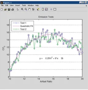
Figure 1-6 shows linear plots of the results of several emission tests of a motor, with a curve fitted to the data.

Figure 1-6.

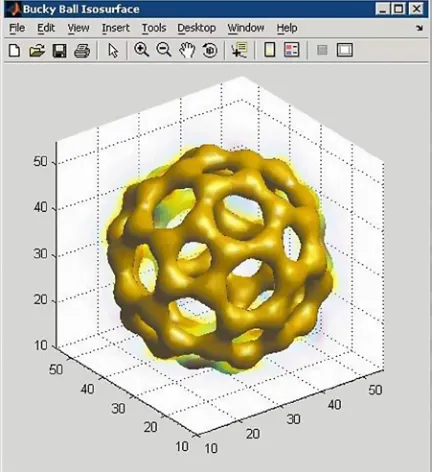
MATLAB also provides functions for displaying two-dimensional arrays, three-dimensional scalar data and three-dimensional vector data. It is possible to use these functions to visualize and understand large amounts of complex multi-dimensional data. It is also possible to define the characteristics of the diagrams, such as the orientation of the camera, perspective, lighting, light source and transparency. Three-dimensional diagramming features include:

Surface, contour and mesh plots

•฀

Space curves

(11)

Figure 1-7.

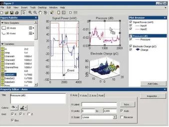
MATLAB includes interactive tools for graphic editing and design. From a MATLAB diagram, you can perform any of the following tasks:

Drag and drop new sets of data into the figure

•฀

Change the properties of any object in the figure

•฀

Change the zoom, rotation, view (i.e. panoramic), camera angle and lighting

•฀

Add data labels and annotations

•฀

Draw shapes

•฀

Generate an M-file for reuse with different data

•฀

(12)

Figure 1-8.

MATLAB is compatible with all the well-known data file and graphics formats, such as GIF, JPEG, BMP, EPS, TIFF, PNG, HDF, AVI, and PCX. As a result, it is possible to export MATLAB diagrams to other applications, such as Microsoft Word and Microsoft Powerpoint, or desktop publishing software. Before exporting, you can create and apply style templates that contain all the design details, fonts, line thickness, etc., necessary to comply with the publication specifications.

Numerical Calculation

MATLAB contains mathematical, statistical, and engineering functions that support most of the operations carried out in those fields. These functions, developed by math experts, are the foundation of the MATLAB language. To cite some examples, MATLAB implements mathematical functions and data analysis in the following areas:

Manipulation of matrices and linear algebra

•฀

Polynomials and interpolation

•฀

Fourier analysis and filters

•฀

Statistics and data analysis

•฀

Optimization and numerical integration

(13)

Publication of Results and Distribution of Applications

In addition, MATLAB contains a number of functions which allow you to document and share your work. You can integrate your MATLAB code with other languages and applications, and distribute your algorithms and MATLAB applications as autonomous programs or software modules.

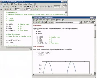
MATLAB allows you to export the results in the form of a diagram or as a complete report. You can export diagrams to all popular graphics formats and then import them into other packages such as Microsoft Word or Microsoft PowerPoint. Using the MATLAB Editor, you can automatically publish your MATLAB code in HTML format, Word, LaTeX, etc. For example, Figure 1-9 shows an M-file (left) published in HTML (right) using the MATLAB Editor. The results, which are sent to the Command Window or to diagrams, are captured and included in the document and the comments become titles and text in HTML.

Figure 1-9.

It is possible to create more complex reports, such as mock executions and various parameter tests, using MATLAB Report Generator (available separately).

MATLAB provides functions enabling you to integrate your MATLAB applications with C and C++ code, FORTRAN code, COM objects, and Java code. You can call DLLs and Java classes and ActiveX controls. Using the MATLAB engine library, you can also call MATLAB from C, C++, or FORTRAN code.

(14)

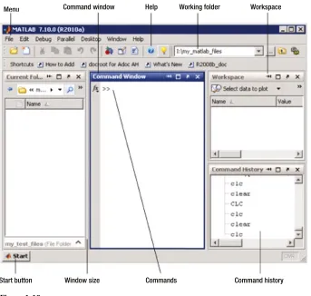
The MATLAB working environment

Figure 1-10 shows the primary workspace of the MATLAB environment. This is the screen in which you enter your MATLAB programs.

Menu Command window Help Working folder Workspace

Start button Window size Commands Command history

Menu

Figure 1-10.

The following table summarizes the components of the MATLAB environment.

Tool

Description

Command History This allows you to see the commands entered during the session in the Command Window, as well as copy them and run them (lower right part of Figure 1-11)

Command Window This is where you enter MATLAB commands (central part of Figure 1-11)

(15)

Figure 1-11.

(16)

CHAPTER 1 ■ INTRODUCING MATLAB AND THE MATLAB WORKING ENVIRONMENT MATLAB commands are written in the Command Window to the right of the user input prompt “»” and the response to the command will appear in the lines immediately below. After exiting from the response, the user input prompt will re-display, allowing you to input more entries (Figure 1-13).

Figure 1-13.

When an input is given to MATLAB in the Command Window and the result is not assigned to a variable, the response returned will begin with the expression “ans=”, as shown near the top of Figure 1-13. If the results are assigned to a variable, we can then use that variable as an argument for subsequent input. This is the case for the variable v in Figure 1-13, which is subsequently used as the input for an exponential.

To run a MATLAB command, simply type the command and press Enter. If at the end of the input we put a semicolon, the program runs the calculation and keeps it in memory (Workspace), but does not display the result on the screen (see the first entry in Figure 1-13). The input prompt “»” appears to indicate that you can enter a new command.

(17)

Descriptive comments can be entered in a command input line by starting them with the “%” symbol. When you run the input, MATLAB ignores the comment and processes the rest of the code (see Figure 1-15).

Figure 1-14.

Figure 1-15.

To simplify the process of entering script to be evaluated by the MATLAB interpreter (via the Command Window prompt), you can use the arrow keys. For example, if you press the up arrow key once, you will recover the last entry you submitted. If you press the up key twice, you will recover the penultimate entry you submitted, and so on.

If you type a sequence of characters in the input area and then press the up arrow key, you will recover the last entry you submitted that begins with the specified string.

(18)

CHAPTER 1 ■ INTRODUCING MATLAB AND THE MATLAB WORKING ENVIRONMENT Below is a summary of the keys that can be used in MATLAB’s input area (command line), together with their functions:

Up arrow (Ctrl-P) Retrieves the previous entry.

Down arrow (Ctrl-N) Retrieves the following entry.

Left arrow (Ctrl-B) Moves the cursor one character to the left.

Right arrow (Ctrl-F) Moves the cursor one character to the right.

CTRL-left arrow Moves the cursor one word to the left.

CTRL-right arrow Moves the cursor one word to the right.

Home (Ctrl-A) Moves the cursor to the beginning of the line.

End (Ctrl-E) Moves the cursor to the end of the current line.

Escape Clears the command line.

Delete (Ctrl-D) Deletes the character indicated by the cursor.

Backspace Deletes the character to the left of the cursor.

CTRL-K Deletes (kills) the current line.

The command clc clears the command window, but does not delete the contents of the work area (the contents remain in the memory).

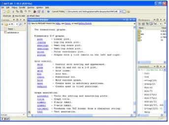
Help in MATLAB

(19)

Figure 1-17.

You can ask for help about a specific command command (Figure 1-18) or on any topic topic (Figure 1-19) by using the command help command or help topic.

(20)

Figure 1-19.

(21)

Numerical Computation with MATLAB

You can use MATLAB as a powerful numerical computer. While most calculators handle numbers only to a preset degree of precision, MATLAB performs exact calculations to any desired degree of precision. In addition, unlike calculators, we can perform operations not only with individual numbers, but also with objects such as arrays.

Most of the topics of classical numerical analysis are treated in this software. It supports matrix calculus, statistics, interpolation, least squares fitting, numerical integration, minimization of functions, linear programming, numerical and algebraic solutions of differential equations and a long list of further numerical analysis methods that we’ll meet as this book progresses.

Here are some examples of numerical calculations with MATLAB. (As we know, to obtain the results it is necessary to press Enter once the desired command has been entered after the prompt “»”.)

1. We simply calculate 4 + 3 to obtain the result 7. To do this, just type 4 + 3, and then Enter.

» 4 + 3

ans =

7

2. We find the value of 3 to the power of 100, without having previously set the precision. To do this we simply enter 3 ^ 100.

» 3 ^ 100

ans =

5. 1538e + 047

3. We can use the command “format long e” to obtain results to 15 digits (floating-point).

» format long e

» 3^100

ans =

5.153775207320115e+047

4. We can also work with complex numbers. We find the result of the operation raising (2 + 3i) to the power 10 by typing the expression (2 + 3i) ^ 10.

» (2 + 3i) ^ 10

ans =

(22)

5. The previous result is also available in short format, using the “format short” command.

» format short » (2 + 3i)^10

ans =

-1.4152e+005- 1.4567e+005i

6. We can calculate the value of the Bessel function J₀ at 11.5. To do this we type besselj(0,11.5).

>> besselj(0,11.5)

ans =

-0.0677

Symbolic Calculations with MATLAB

MATLAB perfectly handles symbolic mathematical computations, manipulating and performing operations on formulae and algebraic expressions with ease. You can expand, factor and simplify polynomials and rational and trigonometric expressions, find algebraic solutions of polynomial equations and systems of equations, evaluate derivatives and integrals symbolically, find solutions of differential equations, manipulate powers, and investigate limits and many other features of algebraic series.

To perform these tasks, MATLAB first requires all the variables (or algebraic expressions) to be written between single quotes. When MATLAB receives a variable or expression in quotes, it is interpreted as symbolic.

Here are some examples of symbolic computations with MATLAB.

1. We can expand the following algebraic expression: ((x+1)(x+2)-(x+2)^2)^3. This is done by typing: expand('(x+1)(x+2)-(x+2)^2)^3'). The result will be another algebraic expression:

» syms x; expand(((x + 1) *(x + 2)-(x + 2) ^ 2) ^ 3)

ans =

-x ^ 3-6 * x ^ 2-12 * x-8

2. We can factor the result of the calculation in the above example by typing: factor(‘((x + 1) *(x + 2)-(x + 2) ^ 2) ^ 3’)

» syms x; factor(((x + 1)*(x + 2)-(x + 2)^2)^3)

(23)

4. We can simplify the previous result:

>> syms x; simplify(int(x^2*sin(x)^2, x))

ans =

sin(2*x)/8 -(x*cos(2*x))/4 -(x^2*sin(2*x))/4 + x^3/6

5. We can present the previous result using a more elegant mathematical notation:

>> syms x; pretty(simplify(int(x^2*sin(x)^2, x)))

ans =

On the other hand, MATLAB can use the Maple program libraries to work with symbolic math, and can thus extend its field of action. In this way, MATLAB can be used to work on such topics as differential forms, Euclidean geometry, projective geometry, statistics, etc.

(24)

Graphics with MATLAB

MATLAB can generate two- and three-dimensional graphs, as well as contour and density plots. You can graphically represent data lists, controlling colors, shading and other graphics features. Animated graphics are also supported. Graphics produced by MATLAB are portable to other programs.

Some examples of MATLAB graphics are given below.

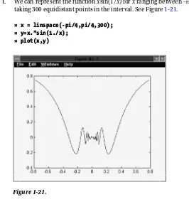
1. We can represent the function xsin(1/x) for x ranging between -p/4 and p/4, taking 300 equidistant points in the interval. See Figure 1-21.

» x = linspace(-pi/4,pi/4,300); » y=x.*sin(1./x);

» plot(x,y)

Figure 1-21.

2. We can give the above graph a title and label the axes, and we can add a grid. See Figure 1-22. » x = linspace(-pi/4,pi/4,300);

» y=x.*sin(1./x); » plot(x,y); » grid;

(25)

Figure 1-22.

3. We can generate a graph of the surface defined by the function z = sin(sqrt(x^2+y^2)) /sqrt(x^2+y^2), where x and y vary over the interval (- 7.5, 7.5), taking equally spaced points 0.5 apart. See Figure 1-23.

» x =-7.5:. 5:7.5; » y = x;

» [X, Y] = meshgrid(x,y);

» Z=sin(sqrt(X.^2+Y.^2))./sqrt(X.^2+Y.^2); » surf(X, Y, Z)

(26)

CHAPTER 1 ■ INTRODUCING MATLAB AND THE MATLAB WORKING ENVIRONMENT These 3D graphics allow you to get a clear picture of figures in space, and are very helpful in

visually identifying intersections between different bodies, and in generating all kinds of space curves, surfaces and volumes of revolution.

4. We can generate the three dimensional graph corresponding to the helix with parametric coordinates: x = sin(t), y = cos(t), z = t. See Figure 1-24.

» t=0:pi/50:10*pi; » plot3(sin(t),cos(t),t)

Figure 1-24.

5. We can represent a planar curve given by its polar coordinates r = cos(2t) * sin(2t) for t varying in the range between 0 and p by equally spaced points 0.01 apart. See Figure 1-25.

» t = 0:. 1:2 * pi;

(27)

6. We can make a graph of a symbolic function using the command “ezplot”. See Figure 1-26. » y ='x ^ 3 /(x^2-1)';

» ezplot(y,[-5,5])

Figure 1-26. Figure 1-25.

(28)

General Notation

As for any program, the best way to learn MATLAB is to use it. By practicing on examples you become familiar with the syntax and notation peculiar to MATLAB. Each example we give consists of the header with the user input prompt “»” followed by the MATLAB response on the next line. See Figure 1-27.

Figure 1-27.

(29)

It is important to pay attention to the use of uppercase versus lowercase letters, parentheses versus square brackets, spaces and punctuation (particularly commas and semicolons).

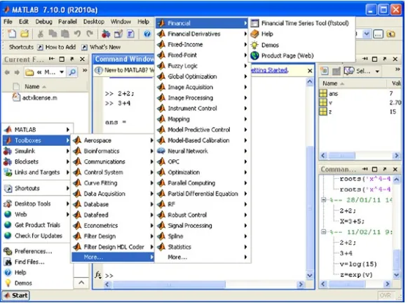
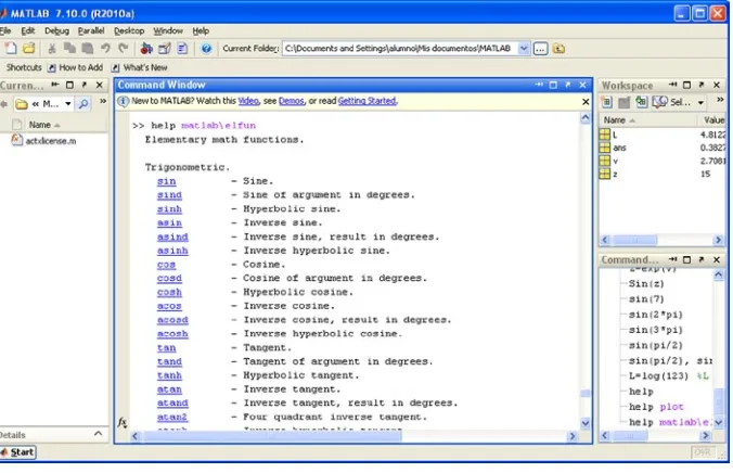
Help with Commands

We have already seen in the previous chapter how you can get help using MATLAB’s drop down menus. But, in addition, support can also be obtained via commands (instructions or functions), implemented as MATLAB objects.

You can use the help command to get immediate access to diverse information.

» help

HELP topics:

matlab\general - General purpose commands.

matlab\ops - Operators and special characters. matlab\lang - Programming language constructs.

matlab\elmat - Elementary matrices and matrix manipulation. matlab\elfun - Elementary math functions.

matlab\specfun - Specialized math functions.

matlab\matfun - Matrix functions - numerical linear algebra. matlab\datafun - Data analysis and Fourier transforms. matlab\polyfun - Interpolation and polynomials. matlab\funfun - Function functions and ODE solvers. matlab\sparfun - Sparse matrices.

matlab\graph2d - Two dimensional graphs. matlab\graph3d - Three dimensional graphs. matlab\specgraph - Specialized graphs. matlab\graphics - Handle Graphics.

matlab\uitools - Graphical user interface tools. matlab\strfun - Character strings.

matlab\iofun - File input/output. matlab\timefun - Time and dates.

matlab\datatypes - Data types and structures.

matlab\winfun - Windows Operating System Interface Files(DDE/ActiveX) matlab\demos - Examples and demonstrations.

toolbox\symbolic - Symbolic Math Toolbox. toolbox\tour - MATLAB Tour

toolbox\local - Preferences.

For more help on directory/topic, type "help topic".

As we can see, the help command displays a list of program directories and their contents. Help on any given topic topic can be displayed using the command help topic. For example:

» help inv

INV Matrix inverse.

(30)

CHAPTER 1 ■ INTRODUCING MATLAB AND THE MATLAB WORKING ENVIRONMENT See also SLASH, PINV, COND, CONDEST, NNLS, LSCOV.

(31)

cplxpair - Sort numbers into complex conjugate pairs.

Rounding and remainder.

There is a command for help on a certain sequence of characters (lookfor string) which allows you to find all those functions or commands that contain or refer to the given string string. This command is very useful when there is no direct support for the specified string, or if you want to view the help for all commands related to the given sequence. For example, if we seek help for all commands that contain the sequence complex, we can use the lookfor complex command to see which commands MATLAB provides.

» lookfor complex

ctranspose.m: %' Complex conjugate transpose. CONJ Complex conjugate.

CPLXPAIR Sort numbers into complex conjugate pairs. IMAG Complex imaginary part.

REAL Complex real part.

CDF2RDF Complex diagonal form to real block diagonal form. RSF2CSF Real block diagonal form to complex diagonal form. B5ODE Stiff problem, linear with complex eigenvalues(B5 of EHL). CPLXDEMO Maps of functions of a complex variable.

CPLXGRID Polar coordinate complex grid. CPLXMAP Plot a function of a complex variable.

GRAFCPLX Demonstrates complex function plots in MATLAB.

ctranspose.m: %TRANSPOSE Symbolic matrix complex conjugate transpose. SMOKE Complex matrix with a "smoke ring" pseudospectrum.

MATLAB and Programming

(32)

CHAPTER 1 ■ INTRODUCING MATLAB AND THE MATLAB WORKING ENVIRONMENT As in programming languages like C or FORTRAN, in MATLAB you can write programs with loops, control flow and conditionals. MATLAB can write procedural programs, i.e., it can define a sequence of standard steps to run. As in C or Pascal, a Do, For, or While loop can be used for repetitive calculations. The language of MATLAB also includes conditional constructs such as If—Then—Else. MATLAB also supports different logical operators, such as AND, OR, NOT and XOR.

MATLAB supports procedural programming (with iterative processes, recursive functions, loops, etc.), functional programming and object-oriented programming. Here are two simple examples of programs. The first generates the Hilbert matrix of order n, and the second calculates all the Fibonacci numbers less than 1000.

% Generating the Hilbert matrix of order n t = '1/(i+j-1)';

% Calculating the Fibonacci numbers f = [1 1]; i = 1;

while f(i) + f(i-1) < 1000 f(i+2) = f(i) + f(i+1); i = i+1 end

Commands to Escape and Exit to the MS-DOS Environment

There are three ways you can escape from the MATLAB Command Window to the MS-DOS operating system environment in order to run temporary assignments. Entering the command ! dos_command in the Command Window allows you to run the specified DOS command in the MATLAB environment. For example:

! dir

(33)

The command ! dos_command & is used to execute the specified DOS command in background mode. The command is executed by opening a DOS environment window on the MATLAB Command Window, as shown in Figure 1-29. To return to the MATLAB environment simply right-click anywhere in the Command Window (the DOS environment window will close automatically). You can return to the DOS window at any time to run any operating system command by clicking the icon labeled MS-DOS symbol at the bottom of the screen.

Figure 1-30. Figure 1-29.

(34)

CHAPTER 1 ■ INTRODUCING MATLAB AND THE MATLAB WORKING ENVIRONMENT The command >>dos dos_command is also used to execute the specified DOS command in automatic mode in the MATLAB Command Window (Figure 1-31).

Figure 1-31.

(35)

CHAPTER 2 First Order Differential Equations.

Exact Equations, Separation of

Variables, Homogeneous and

Linear Equations

First Order Differential Equations

Although it implements only a relatively small number of commands related to this topic, MATLAB’s treatment of differential equations is nevertheless very efficient. We shall see how we can use these commands to solve each type of differential equation algebraically. Numerical methods for the approximate solution of equations and systems of equations are also implemented.

The basic command used to solve differential equations is dsolve. This command finds symbolic solutions of ordinary differential equations and systems of ordinary differential equations. The equations are specified by symbolic expressions where the letter D is used to denote differentiation, or D2, D3, etc, to denote differentiation of order 2,3,…, etc. The letter preceded by D (or D2, etc) is the dependent variable (which is usually y), and any letter that is not preceded by D (or D2, etc) is a candidate for the independent variable. If the independent variable is not specified, it is taken to be x by default. If x is specified as the dependent variable, then the independent variable is

t. That is, x is the independent variable by default, unless it is declared as the dependent variable, in which case the independent variable is understood to be t.

You can specify initial conditions using additional equations, which take the form y(a) = b or Dy(a) = b,…, etc. If the initial conditions are not specified, the solutions of the differential equations will contain constants of

integration, C1, C2,…, etc. The most important MATLAB commands that solve differential equations are the following:

dsolve(‘equation’, ‘v’): This solves the given differential equation, where v is the independent variable (if ‘v’ is not specified, the independent variable is x by default). This returns only explicit solutions.

dsolve(‘equation’, ‘initial_condition’,…, ‘v’): This solves the given differential equation subject to the specified initial condition.

dsolve(‘equation’, ‘cond1’, ‘cond2’,…, ‘condn’, ‘v’): This solves the given differential equation subject to the specified initial conditions.

dsolve(‘equation’, ‘cond1, cond2,…, condn’, ‘v’): This solves the given differential equation subject to the specified initial conditions.

(36)

CHAPTER 2 ■ FIRST ORDER DIFFERENTIAL EQUATIONS. EXACT EQUATIONS, SEPARATION OF VARIABLES, HOMOGENEOUS AND LINEAR EQUATIONS

dsolve(‘eq1, eq2,…, eqn’, ‘cond1, cond2,…, condn’ , ‘v’): This solves the given system of differential equations subject to the specified initial conditions.

maple(‘dsolve(equation, func(var))’): This solves the given differential equation, where var is the independent variable and func is the dependent variable (returns implicit solutions).

maple(‘dsolve({equation, cond1, cond2,… condn}, func(var))’): This solves the given differential equation subject to the specified initial conditions.

maple(‘dsolve({eq1, eq2,…, eqn}, {func1(var), func2(var),… funcn(var)})’): This solves the given system of differential equations (returns implicit solutions).

maple(‘dsolve(equation, func(var), ’explicit’)’): This solves the given differential equation, offering the solution in explicit form, if possible.

Examples are given below.

First, we solve differential equations of first order and first degree, both with and without initial values.

» pretty(dsolve('Dy = a*y'))

C2 exp(a t)

» pretty(dsolve('Df = f + sin(t)'))

sin(t) cos(t) C6 exp(t) - - 2 2

The previous two equations can also be solved in the following way:

» pretty(sym(maple('dsolve(diff(y(x), x) = a * y, y(x))')))

y(x) = exp(a x) _C1

Now we solve an equation of second degree and first order.

(37)

CHAPTER 2 ■ FIRST ORDER DIFFERENTIAL EQUATIONS. EXACT EQUATIONS, SEPARATION OF VARIABLES, HOMOGENEOUS AND LINEAR EQUATIONS We can also solve this in the following way:

» pretty(maple('dsolve({diff(y(s),s)^2 + y(s)^2 = 1, y(0) = 0}, y(s))'))

y(s) = sin(s), y(s) = - sin(s)

Now we solve an equation of second order and first degree.

» pretty(dsolve('D2y = - a ^ 2 * y ', 'y(0) = 1, Dy(pi/a) = 0'))

exp(-a t i) exp(a t i) - + 2 2

Next we solve a couple of systems, both with and without initial values.

>> dsolve('Dx = y', 'Dy = -x')

>> y=dsolve('Df = 3*f+4*g', 'Dg = -4*f+3*g')

(38)

>> y=dsolve('Df = 3*f+4*g, Dg = -4*f+3*g', 'f(0)=0, g(0)=1')

y =

This last system can also be solved in the following way:

» pretty(maple('dsolve({diff(f(x),x)= 3*f(x)+4*g(x), diff(g(x),x)=-4*f(x)+3*g(x), f(0)=0,g(0)=1}, {f(x),g(x)})'))

{f(x) = exp(3 x) sin(4 x), g(x) = exp(3 x) cos(4 x)}

Separation of Variables

A differential equation is said to have separable variables if it can be written in the form

f x dx g y dy( ) = ( ) .

This type of equation can be solved immediately by putting

ò

f x dx( ) =

ò

g y dy c( ) + .

(39)

EXERCISE 2-1

Solve the differential equation:

ycos( )x dx- +(1 y dy2) =0, ( )y0 =1.

First of all we try to solve it directly. The equation can be written in the form:

y x x y x exp(C33 + t*cos(x))*exp(-wrightOmega(2*C33 + 2*t*cos(x))/2)

Thus the differential equation appears not to be solvable with

dsolve

. However, in this case, the variables are

separable, so we can solve the equation as follows:

» pretty(solve('int(cos(x), x) = int((1+y^2) / y, y)'))

+- -+

Thus, after a little rearrangement, we see that the general solution is given by:

sin( ) log( )x = y +1 2/ y2+C.

(40)

The above differential equation is also solvable directly by using:

» pretty(maple('dsolve(diff(y(x), x) = y(x) * cos(x) /(1 + y(x) ^ 2), y(x))'))

2

log(y(x)) + 1/2 y(x) - sin(x) = _C1

Homogeneous Differential Equations

Consider a general differential equation of first degree and first order of the form

M x y dx N x y dy( , ) = ( , ) .

This equation is said to be homogeneous of degree n if the functions M and N satisfy:

M tx ty t M x y

For this type of equation, we can transform the initial differential equation (with variables x and y), via the change of variable x = vy, into another (separable) equation (with variables v and y). The new equation is solved by separation of variables and then the solution of the original equation is found by reversing the change of variable.

EXERCISE 2-2

Solve the differential equation:

(x2_-y dx x y dy2) ₊ ₌₀.

First we check if the equation is homogeneous

(41)

Before performing the change of variable, it is advisable to load the library

difforms

, using the command

maple(‘with(difforms)’), which will allow you to work with differential forms. Once this library is loaded it is

also convenient to use the command maple(‘defform(v=0,x=0,y=0)’), which allows you to declare all variables

which will not be constants or parameters in the differentiation.

» maple('with(difforms)');

The previous expression can be simplified.

» pretty(maple('convert(collect(((v^2*y^3-y^3) * d(v) + v ^ 3 * y ^ 2 * d(y)) /(v^3*y^3), {d(v), d(y)}), parfrac, y)'))

2

(42)

Now, we solve the equation:

» pretty(simple('int((v^2-1)/v ^ 3, v) + int(1/y,y)'))

1

log(v) + ---- + log(y) 2

2 v

Finally we reverse the change of variable:

» pretty(simple('subs(v = x / y log(v) + 1/2/v ^ 2 + log(y))'))

2 y log(x) + 1/2 2 x

Thus the general solution of the original differential equation is:

log( )x y .

x C

+1 =

2 2

2

Now we can represent the solutions of this differential equation graphically. To do this we graph the solutions with

parameter C, which is equivalent to the following contour plot of the function defined by the left-hand side of the

above general solution (see Figure 18-1):

» [x,y]=meshgrid(0.1:0.05:1/2,-1:0.05:1); » z=y.^2./(2*x.^2)+log(x);

(43)

Exact Differential Equations

The differential equation

M x y dx N x y dy( , ) + ( , ) =0

is said to be exact if ¶ ¶ =¶N x M y¶ . If the equation is exact, then there exists a function F such that its total differential

dF coincides with the left-hand side of the above equation, i.e.:

dF M x y dx N x y dy= ( , ) + ( , )

therefore the family of solutions is given by F(x,y) = C.

The exercise below follows the usual steps of an algebraic solution to this type of equation.

EXERCISE 2-3

Solve the differential equation:

- + +

(

1 y exy y_cos(xy dx₎

)

+ +

(

1 x exy+x_cos(xy dy₎

)

=0

First of all, we try to solve the equation with

dsolve

:

» maple('m:=(x,y) - > - 1 + y * exp(x*y) + y * cos(x*y)'); » maple('n:=(x,y) - > 1 + x * exp(x*y) + x * cos(x*y)'); » dsolve('m(x,y) + n(x,y) * Dy = 0')

??? Error using ==> dsolve

Explicit solution could not be found.

Thus the function

dsolve

does not give a solution to the proposed equation. We are going to try to solve the

equation using the classical algebraic method.

First we check that the proposed differential equation is exact.

» pretty(simple(diff('m(x,y)','y')))

exp(y x) + x y exp(y x) + cos(y x) - x sin(y x) y

» pretty(simple(diff('n(x,y)','x')))

exp(y x) + x y exp(y x) + cos(y x) - x sin(y x) y

Since the equation is exact, we can find the solution in the following way:

» solution1 = simplify('int(m(x,y), x) + g(y)')

solution1 =

(44)

Now we find the function

g

(

y

) via the following condition:

diff int( ( , ), )

(

m x y x +g y y( ),

)

=n x y( , )

» pretty(simplify('int(m(x,y), x) + g(y)'))

-x + exp(y x) + sin(y x) + g(y)

» pretty(simplify('diff(-x+exp(y*x) + sin(y*x) + g(y), y)'))

d x exp(y x) x + x cos(y x) + -- g(y) dy

» simplify('solve(x * exp(y*x) + x * cos(y*x) + diff(g(y), y) = n(x,y), diff(g(y), y))')

ans =

1

Thus

g

'(

y

) = 1, so the final solution will be, omitting the addition of a constant:

» pretty(simplify('subs(g(y) = int(1,y),-x+exp(y*x) + sin(y*x) + g(y))'))

-x + exp(y x) + sin(y x) + y

To graphically represent the family of solutions, we draw the following contour plot of the above expression

(Figure 18-2):

(45)

Figure 2-2.

In the following section we will see how any reducible differential equation can be transformed to an exact

equation using an integrating factor.

Linear Differential Equations

A linear first order differential equation is an equation of the form:

dy dx P x y Q x+ ( ) = ( )

where P(x) and Q(x) are given functions of x.

Differential equations of this type can be transformed into exact equations by multiplying both sides of the equation by the integrating factor:

eòP x dx( ) and the general solution is then given by the expression:

e-òP x dx e P x dxQ x dx

æ è

ç ( ) ö_ø÷æ_èç

ò

ò ( ) ( ) ö_ø÷

(46)

EXERCISE 2-4

Solve the differential equation:

x dy dx+3y x= sin( ).x

» pretty(simple(dsolve('x * Dy + 3 * y = x * sin(x)')))

(47)

CHAPTER 3 Higher Order Differential Equations.

The Laplace Transform and Special

Types of Equations

Ordinary High-Order Equations

An ordinary linear differential equation of ordern has the following general form:

k

If the function f (x) is identically zero, the equation is called homogeneous. Otherwise, the equation is called

non-homogeneous. If the functions a_i(x) (i = 1, …, n) are constant, the equation is said to have constant coefficients. A concept of great importance in this context is that of a set of linearly independent functions. A set of functions { f₁(x), f₂(x), …, f_n(x)} is linearly independent if, for any x in their common domain of definition, the Wronskian

determinant of the functions is non-zero. The Wronskian determinant of the given set of functions, at a point x of their common domain of definition, is defined as follows:

f x

The MATLAB command maple(‘Wronskian’) allows you to calculate the Wronskian matrix of a set of functions. Its syntax is:

maple(‘Wronskian(V,x)’): This computes the Wronskian matrix corresponding to the vector of functions V with independent variable x.

A set S = { f₁(x), …, f_n(x)} of linearly independent non-trivial solutions of a homogeneous linear equation of order n

a x y x a x y x a x y x a x y_n n x

0

( ) ( )

+ 1

( ) ( )

+ 2

( ) ( )

+×××+

( )

=0

( )

¢ ²

(48)

CHAPTER 3 ■ HIGHER ORDER DIFFERENTIAL EQUATIONS. THE LAPLACE TRANSFORM AND SPECIAL TYPES OF EQUATIONS

If the functions a_i(x) (i = 1, …, n) are continuous in an open interval I, then the homogeneous equation has a set of fundamental solutions S = {f_i(x)} in I.

In addition, the general solution of the homogeneous equation will then be given by the function:

f x c f x

where {c_i} is a set of arbitrary constants. The equation:

is called the characteristic equation of the homogeneous differential equation with constant coefficients. The solutions of this characteristic equation determine the general solutions of the corresponding differential equation.

EXERCISE 3-1

Show that the set of functions

{ex,xex,x e2 x}

is linearly independent.

» indfunctions = maple('vector([exp(x), x * exp(x), x ^ 2 * exp(x)])')

indfunctions =

(49)

Linear Higher-Order Equations. Homogeneous Equations with

Constant Coefficients

The homogeneous linear differential equation of order n

k characteristic equation determine the general solution of the associated differential equation.

If the mi (i = 1, …, n) are all different, the general solution of the homogeneous equation with constant

If some m_i is a root of multiplicity k of the characteristic equation, then it determines the following k terms of the solution: These two roots determine a pair of terms in the general solution of the homogeneous equation:

c e_j ax bx c e bx

j ax

cos

( )

+ ₊₁ sin

( )

.

MATLAB directly applies this method to obtain the solutions of homogeneous linear equations with constant coefficients, using the command dsolve or maple(‘dsolve’).

(50)

Looking at the solution, it is evident that the characteristic equation has two pairs of complex conjugate solutions.

» solve('9*x^4-6*x^3+46*x^2-6*x+37=0')

Non-Homogeneous Equations with Constant Coefficients.

Variation of Parameters

Consider the non-homogeneous linear equation with constant coefficients:

(51)

CHAPTER 3 ■ HIGHER ORDER DIFFERENTIAL EQUATIONS. THE LAPLACE TRANSFORM AND SPECIAL TYPES OF EQUATIONS A particular solution of the non-homogeneous equation is given by:

yp x u x y x

where the functions u_i(x) are obtained as follows:

u x f x W y x y x y x

The solution of the non-homogeneous equation is then given by combining the general solution of the homogeneous equation with the particular solution of the non-homogeneous equation. If the roots m_i of the characteristic equation of the homogeneous equation are all different, the general solution of the non-homogeneous equation is:

y x c em x c em x c e y x

If some of the roots are repeated, we refer to the general form of the solution of a homogeneous equation discussed earlier.

EXERCISE 3-4

Solve the following differential equations:

y'' y' y x

x

+4 +13 = _cos2

( )

3 _,

y''-₂y'+ =y ex

( )

x

ln .

We will follow the algebraic method of variation of parameters to solve the first equation. We first consider the

characteristic equation of the homogeneous equation to obtain a set of linearly independent solutions.

(52)

We see that the Wronskian is non-zero, indicating that the functions are linearly independent. Now we calculate

the functions

W

_i

(

x

),

i

= 1, 2.

» maple('W1: x-= > array([[0, y2(x)], [1, diff((y2)(x), x)]])'); » pretty(simplify(maple('det(W1(x))')))

-exp(-2 x) sin(3 x)

» maple('W2: x-= > array([[y1(x), 0], [diff((y1)(x), x), 1]])'); » pretty(simplify(maple('det(W2(x))')))

exp(-2 x) cos(3 x)

Now we calculate the particular solution of the non-homogeneous equation.

» maple('u1:=x->factor(simplify(int(f(x)*det(W1(x))/det(W(x)),x)))'); » maple('u1(x)')

ans =

1/14652300*exp(2*x)*(129285*cos(9*x)*x-6084*cos(9*x)-28730*sin(9*x)*x-13013*sin(9*x)+281775*cos(3*x)*x-86700*cos(3*x)-187850*sin(3*x)*x-36125*sin(3*x))

» maple('u2:=x->factor(simplify(int(f(x)*det(W2(x))/det(W(x)),x)))'); » maple('u2(x)')

ans =

1/14652300 * exp(2*x) *(563550 * cos(3*x) * x+108375 * cos(3*x) + 845325 * sin(3*x) * x-260100 * sin(3*x) + 28730 * cos(9*x) * x+13013 * cos(9*x) + 129285 * sin(9*x) * x-6084 * sin(9*x))

» maple('yp: = x - > factor(simplify(y1(x) *(x) u1 + y2(x) * u2(x)))'); » maple('yp(x)')

ans =

-23/1105 * x * cos(3*x) ^ 2 + 13436/1221025 * cos(3*x) ^ 2 + 24/1105 * cos(3*x) * sin(3*x) * x + 3852/1221025 * cos(3*x) * sin(3*x) + 54/1105 * x-21168/1221025

Then we can write the general solution of the non-homogeneous equation:

» maple(' y: = x - > simplify(c1 * y1(x) + c2 * y2(x) + yp(x))'); » maple('combine(and(x), trig)')

(53)

Figure 3-1.

» fplot(simplify('subs(c1=-5,c2=-4,y(x))'),[-1,1]) » hold on

» fplot(simplify('subs(c1=-5,c2=4,y(x))'),[-1,1]) » fplot(simplify('subs(c1=-5,c2=2,y(x))'),[-1,1]) » fplot(simplify('subs(c1=-5,c2=-2,y(x))'),[-1,1]) » fplot(simplify('subs(c1=-5,c2=-1,y(x))'),[-1,1]) » fplot(simplify('subs(c1=-5,c2=1,y(x))'),[-1,1]) » fplot(simplify('subs(c1=5,c2=1,y(x))'),[-1,1]) » fplot(simplify('subs(c1=5,c2=-1,y(x))'),[-1,1]) » fplot(simplify('subs(c1=5,c2=-2,y(x))'),[-1,1]) » fplot(simplify('subs(c1=5,c2=2,y(x))'),[-1,1]) » fplot(simplify('subs(c1=5,c2=4,y(x))'),[-1,1]) » fplot(simplify('subs(c1=5,c2=-4,y(x))'),[-1,1]) » fplot(simplify('subs(c1=0,c2=-4,y(x))'),[-1,1]) » fplot(simplify('subs(c1=0,c2=4,y(x))'),[-1,1]) » fplot(simplify('subs(c1=0,c2=2,y(x))'),[-1,1]) » fplot(simplify('subs(c1=0,c2=-2,y(x))'),[-1,1]) » fplot(simplify('subs(c1=0,c2=-1,y(x))'),[-1,1]) » fplot(simplify('subs(c1=0,c2=1,y(x))'),[-1,1])

For the second differential equation we directly apply

dsolve

, obtaining the solution:

» pretty(simple(dsolve('D2y-2 * Dy + y = exp(x) * log(x)')))

(54)

Non-Homogeneous Equations with Variable Coefficients.

Cauchy–Euler Equations

A non-homogeneous linear equation with variable coefficients of the form

k

is called a Cauchy–Euler equation.

MATLAB can solve this type of equation directly with the command dsolve or maple(‘dsolve’).

EXERCISE 3-5

Solve the following differential equation:

x y3 ''''₊₁₆x y2 ''₊₇₉xy'₊₁₂₅y₌₀_.

MATLAB provides the commands maple(‘laplace’) and maple(‘invlaplace’) to calculate the Laplace transform and inverse Laplace transform of an expression with respect to a variable. Its syntax is as follows:

maple(‘laplace(expression, t, s)’): This calculates the Laplace transform of a given expression with respect to t. The transformed variable is s.

(55)

CHAPTER 3 ■ HIGHER ORDER DIFFERENTIAL EQUATIONS. THE LAPLACE TRANSFORM AND SPECIAL TYPES OF EQUATIONS Here are some examples.

» pretty(maple('laplace(t^(3/2)-exp(t)+sinh(a*t), t, s)'));

The Laplace transform and its inverse are used to solve certain differential equations. The method is to calculate the Laplace transform of each term of the equation to obtain a new differential equation, which we then solve. Finally, we find the solution of the original equation by applying the inverse Laplace transform to the solution just found.

MATLAB provides the ‘laplace’ option in the maple(‘dsolve’) command, which forces the program to solve the differential equation using the Laplace transform method. The syntax is as follows:

maple('dsolve(equation, func(var), 'laplace')')

EXERCISE 3-6

Solve the differential equation

y'' y' y x e x y y'

+₂ +₄ = - - _,

( )

₀ =₁_,

( )

₀ =₁

using the Laplace transform method.

(56)

We then solve the Laplace transformed differential equation:

» pretty(simplify(maple('solve(L(s)=L1(s),laplace(y(x),x,s))')))

Now we substitute the given initial conditions into the solution.

» maple('TL:=s->solve(L(s)=L1(s),laplace(y(x),x,s))');

This gives the solution of the Laplace transformed equation. To calculate the solution of the original equation we

calculate the inverse Laplace transform of the solution obtained in the previous step.

» maple('TL0:=s->simplify('subs(y(0)=1,(D(y))(0)=1,TL(s))')');

This gives the solution of the original differential equation.

We could also have solved it directly via:

» pretty(simple(sym(maple('dsolve({diff(y(x),x$2)+2*diff(y(x),x)+4*y(x) = x-exp(-x), y(0)=1,D(y) (0)=1},y(x),laplace)'))))

(57)

An example of an orthogonal family of functions (i.e. such that any two distinct functions in the family are orthogonal) is given by:

f

_n

(

x

) = sin(

nx

) and

g

_n

(

x

) = cos(

nx

),

n

= 1, 2, 3, …, in the interval [−

p

,

p

].

MATLAB provides a broad list of orthogonal polynomials, which are very useful in solving certain non-linear differential equations of higher order. The functions that allow us to work with these polynomials are the following:

T(n,x), Chebychev polynomials of the first kind.

U(n,x), Chebychev polynomials of the second kind.

P(n,x), Legendre polynomials.

Now let us look at their relationship to differential equations. It is precisely this relationship which allows us to find solutions of some non-linear equations of higher order. To use these functions we first need to run maple(‘with orthopoly’).

Chebychev Polynomials of the First and Second Kind

The Chebychev polynomials of the first kind are defined as the solutions T_n(x) of the differential equation:

1_- 2 2 0 0 1 2

(

x

)

y’’-x y n y’ + = _,n= _{, , ,}¼

Their orthogonality is given by the weighted inner product:

-

ò

(

-

)

The Chebychev polynomials of the second kind U_n(x) are special cases of the Jacobi polynomials (see below) with a = b = 1/2. They satisfy the orthogonality relationship:

(58)

Legendre Polynomials

The Legendre polynomials P_n(x) are solutions of the Legendre differential equation:

1_- 2 2 1 0

(

x

)

y’’- x y n n’ +

(

+

)

y= _.

Their orthogonality is given by the relation

-

ò

The solutions of the differential equation

1 2 1

are called associated Legendre polynomials. Their orthogonality is given by the relation

P P_km

The solutions H_n(x) of the Hermite differential equation

y’’_-₂x y’ ₊₂ny₌₀

are known as Hermite polynomials.

-¥

The solutions L_n(x) of the general Laguerre differential equation

xy’’₊

(

a_{+ -}₁ x y

)

’₊ny₌₀

are known as generalized Laguerre polynomials.

(59)

Laguerre Polynomials

The solutions of the Laguerre differential equation

x y’’ _{+ -}

(

₁ x y

)

’₊ny₌₀

are known as Laguerre polynomials. This is the particular case a = 0 of the generalized Laguerre polynomials.

Jacobi Polynomials

The solutions of the Jacobi differential equation

1_- 2 2 1 0

(

x

)

y’’+

(

b a- -

(

a b+ +

)

x y

)

’+n n a b

(

+ + +

)

_y=

are known as Jacobi polynomials.

-

ò

The solutions of the Gegenbauer differential equation

1_- 2 2 1 2 0

(

x

)

y’’+

(

a+

)

xy’+n n

(

+ a y

)

=

are known as Gegenbauer polynomials.

(60)

-CHAPTER 3 ■ HIGHER ORDER DIFFERENTIAL EQUATIONS. THE LAPLACE TRANSFORM AND SPECIAL TYPES OF EQUATIONS

EXERCISE 3-7

Find the solutions to the following differential equations:

(1_-_{x y}2) ''_-_xy'₊49_y₌0,

The linearly independent solutions of the following second order differential equation are called Airy functions:

y

"

−

xy

= 0 (Airy equation)

The linearly independent solutions of the following second order differential equation are called Bessel functions:

2 0

(Bessel equation)

(61)

CHAPTER 3 ■ HIGHER ORDER DIFFERENTIAL EQUATIONS. THE LAPLACE TRANSFORM AND SPECIAL TYPES OF EQUATIONS MATLAB implements the following related functions:

Ai(z) and Bi(z) are the linearly independent solutions of the Airy differential equation.

BesselJ(n,z) and BesselY(n,z) are the linearly independent solutions of the Bessel differential equation.

BesselI(n,z) and BesselK(n,z) are the linearly independent solutions of the modified Bessel differential equation.

EXERCISE 3-8

Find the solutions of the differential equation

x y2 xy x2 1 y

4 0

''₊ '₊æ

-è

ç ö_ø÷ = .

The equation is the Bessel differential equation with n = 1/2. We obtain two linearly independent solutions

as follows:

» pretty(simple(maple('BesselJ(1/2,x)')))

1/2 2 sin(x) 1/2 1/2 pi x

» pretty(simple(maple('BesselY(1/2,x)')))

1/2

(62)

CHAPTER 4 Differential Equations Via

Approximation Methods

Higher Order Equations and Approximation Methods

When the known algebraic methods for solving differential equations and systems of differential equations offer no solution, we usually resort to methods of approximation. The approximation methods can involve both symbolic and numerical work. The symbolic approach yields approximate algebraic solutions, and its most representative technique is the Taylor series method. The numerical approach yields a solution in the form of a finite set of solution points, to which a curve can be fitted by various algebraic methods (interpolation, regression,…). This curve will be an approximate solution of the differential equation. Among the most common numerical methods is the Runge–Kutta method.

Approximation methods are most commonly employed to find the solution of equations and systems of differential equations of order and degree greater than one, where the exact solution cannot be obtained by other methods.

The Taylor Series Method

This method provides approximate polynomial solutions of general differential equations, and is based on the Taylor series expansion of functions. MATLAB offers the option ‘series’ for the command maple(‘dsolve’), which allows you to solve equations by this method. Its syntax is as follows:

maple('dsolve(equation, func(var), 'series'))

There is also the command maple(‘powsolve’), which gives a power series solution of linear differential equations, and whose syntax is as follows:

maple('powseries [powsolve](equation, cond1,...,condn) ')

(63)

CHAPTER 4 ■ DIFFERENTIAL EQUATIONS VIA APPROXIMATION METHODS

EXERCISE 4-1

Solve the following two equations by the Taylor series method:

4_{x y}2 _"₊4_xy_’₊₍_x2 _-1₎_y₌0_,

yy"+( ’)y 2+ =₁ ₀,with the initial conditions y( )₀ +₁and y’( )₀ =₁.

» pretty(simple(maple('dsolve(4 * x ^ 2 * diff(y(x), x$ 2) + 4 * x * diff(y(x), x) +(x ^ 2-1) * y(x) = 0 y(x), series)')))

2 4 6 6 y(x) = (_C1 x(1 - 1/24 x + 1/1920 x + O(x )) + _C2 log(x)(O(x ))

2 4 6 / 1/2 + _C2(1 - 1/8 x + 1/384 x + O(x ))) / x

» pretty(simplify(maple('convert(_C1 * x ^(1/2) *(1-1 / 24 * x ^ 2 + 1/1920 * x ^ 4 + O(x^6)) + _C2 *(1/x ^(1/2) * log(x) *(O(x^6)) + 1/x ^(1/2) *(1-1 / 8 * x ^ 2 + 1/384 * x ^ 4 + O(x^6))), polynom)')))

3 5 6 1/1920(1920 _C1 x - 80 x _C1 + _C1 x + 1920 _C1 x o(x))

6 2 4 + 1920 _C2 log(x) o(x) + 1920 _C2 - 240 _C2 x + 5_C2 x

6 1/2 (+1920 _C2 o(x)) / x

» pretty(maple('dsolve({y(x) * diff(y(x), x$ 2) + diff(y(x), x) ^ 2 + 1 = 0, y(0) = 1, D(y)(0) = 1}, y(x), series)'))

(64)

EXERCISE 4-2

Solve the following two systems of equations using the Taylor series method:

(65)

The Runge–Kutta Method

The Runge–Kutta method gives a set of data points to which you can fit a curve, approximating the solution of a differential equation. Maple provides the option numeric for the command maple(‘solve’) which enables the calculation of approximate numerical solutions of differential equations. Its syntax is:

maple('dsolve(equation, func(var), 'numeric'))

EXERCISE 4-3

Solve the following equation using the Runge–Kutta method:

3_{( ")}_y 2 ₌_y_{’’’ ’}_{y with the initial conditions y}_{’( )}0 ₌_y_{"( )}0 ₌1

_.

» maple('f: = dsolve({3 * diff(y(x), x$ 2) ^ 2 = diff(y(x), x$ 3) * diff(y(x), x), y(0) = 1/2, D(y) (0) = 1,(D@@2)(y)(0) = 1}, y(x), numeric)')

ans =

f := proc(x) `dsolve/numeric/result2`(x,3879004,[3]) end

Now, in order to graph the solution, we calculate various points of the solution function

f

generated above

(see Figure

4-1

).

» [maple('f(-0.3)'),maple('f(-0.2)'),maple('f(-0.1)'),maple('f(0)'), maple('f(0.1)'), maple('f(0.2)'),maple('f(0.3)')]

ans =

{x = -.3,y(x) = .2350889359260396}{y(x) = .3167840433732281, x = -.2} {y(x) = .4045548849869109, x = -.1}{y(x) = .5000000000000000, x = 0} {x = .1, y(x) = .6055728090006967}{y(x) = .7254033307597474, x = .2} {y(x) = .8675444679682489, x = .3000000000000000}

» y = [.2350889359260396,.3167840433732281,.4045548849869109,.5,.6055728090006967, .7254033307597474,.8675444679682489];

(66)

Figure 4-1.

We find the degree 2 polynomial which is the best fit to the set of solution points. The equation of this parabola will

be an approximate solution of the differential equation.

» pretty(vpa(poly2sym(polyfit((-0.3:.1:0.3),y,2))))

2

.5747427827483573 x + 1.041293962469090 x +.4991457846921903