A Solution Manual and Notes for:
Statistics and Data Analysis for
Financial Engineering
by David Ruppert
John L. Weatherwax
∗December 21, 2009
Chapter 12 (Regression: Basics)
R Lab
See the R script Rlab.R for this chapter. We plot a pairwise scatter plot of the variables of
interest in Figure 1. From that plot we see that it looks like the strongest linear relationship
exists between consumption and dpi and unemp. The variables cpi and government don’t
seem to be as linearly related to consumption. There seem to be some small outliers in
several variables namely: cpi(for large values),government(large values), andunemp(large
values). There does not seem to be too much correlation between the variable in that none of the scatter plots seem to look strongly linear and thus there does not look to be collinearity problems.
If we fit a linear model on all four variables we get
Call:
lm(formula = consumption ~ dpi + cpi + government + unemp, data = MacroDiff)
Coefficients:
Estimate Std. Error t value Pr(>|t|)
(Intercept) 14.752317 2.520168 5.854 1.97e-08 ***
dpi 0.353044 0.047982 7.358 4.87e-12 ***
cpi 0.726576 0.678754 1.070 0.286
government -0.002158 0.118142 -0.018 0.985
unemp -16.304368 3.855214 -4.229 3.58e-05 ***
Residual standard error: 20.39 on 198 degrees of freedom
Multiple R-squared: 0.3385, Adjusted R-squared: 0.3252
F-statistic: 25.33 on 4 and 198 DF, p-value: < 2.2e-16
The two variables suggested to be the most important above namely dpi and unemp have
the most significant regression coefficients. The anova command gives the following
> anova(fitLm1)
Analysis of Variance Table
Response: consumption
Df Sum Sq Mean Sq F value Pr(>F)
dpi 1 34258 34258 82.4294 < 2.2e-16 ***
cpi 1 253 253 0.6089 0.4361
government 1 171 171 0.4110 0.5222
The anova table emphasizes the facts that when we add cpi and government to the
re-gression of consumption on dpi we don’t reduce the regression sum of square significantly
enough to make a difference in the modeling. Since two of the variables don’t look promising
in the modeling of consumption we will consider dropping them usingstepAIC in theMASS
library. The stepAIC suggests that we should first drop government and thencpifrom the
regression.
Comparing the AIC for the two models gives that the reduction in AIC is 2.827648 starting with an AIC of 1807.064. This does not seem like a huge change.
The two different vifgive
> vif(fitLm1)
dpi cpi government unemp
1.100321 1.005814 1.024822 1.127610
> vif(fitLm2)
dpi unemp
1.095699 1.095699
Note that after removing the two “noise” variables the variance inflation factors of the remaining two variables decreases (as it should) since now we can determine the coefficients with more precision.
Exercises
Exercise 12.1 (the distributions in regression)
Part (a):
Yi∼ N(1.4 + 1.7,0.3) = N(3.1,0.3).
To compute P(Yi ≤ 3|Xi = 1) in R this would be pnorm( 3, mean=3.1, sd=sqrt(0.3) )
to find 0.4275661.
Part (b): We can compute the density of P(Yi=y) as
when we integrate with Mathematica. Here σ1 =
√
0.3 and σ2 =
√
0.7. Thus this density is
consumption
−50 0 50 100 −20 0 20 40 60
−50
0
50
−50
0
50
100
150
dpi
cpi
0
2
4
6
8
10
−20
0
20
40
60
government
−50 0 50 0 2 4 6 8 10 −1.0 0.0 1.0
−1.0
0.0
0.5
1.0
1.5
unemp
Exercise 12.2 (least squares is the same as maximum likelihood)
Maximum likelihood estimation would seek parameters β0 and β1 to maximize the
log-likelihood of the parameters given the data. For the assumptions in this problem this becomes
LL = log
N
Y
i=1
p(Yi|Xi)
!
=Xlogp(Yi|Xi)
=Xlog
1
√
2πσǫ
exp
−(yi−β0−β1xi) 2
2σ2
ǫ
= a constant− 1
2σ2
ǫ
X
i
(yi−β0−β1xi)
2
.
This later summation expression is what we are minimizing when we perform least-squares minimization.
Exercise 12.4 (the VIF for centered variables)
In theR codechap 12.R we perform the requested experiment and if we denote the variable
X−X¯ asV we find
[1] "cor(X,X^2)= 0.974" [1] "cor(V,V^2)= 0.000"
[1] "VIF for X and X^2= 9.951"
[1] "VIF for (X-barX) and (X-barX)^2= 1.000"
Thus we get a very large reduction in the variance inflation factor when we center our variable.
Exercise 12.5 (the definitions of some terms in linear regression)
In this problem we are told that n = 40 and that the empirical correlation r(Y,Yˆ) = 0.65.
Using these facts and the definitions provided in the text we can compute the requested expressions.
Part (a): R2
=r2
YYˆ = (0.65)
2
= 0.4225
Part (b): From the definition of R2 we can write
R2 = 1− residual error SS
Since we know the value of R2 and that the total sum of squares, given by,
total SS =X
i
(Yi−Y¯)
2
,
is 100 we can solve Equation 1 for the residual sum of square. We find we have a residual error sum of squares given by 57.75.
Part (c): Since we can decompose the total sum of squares into the regression and residual
sum of squares as
total SS = regression SS + residual SS, (2)
and we know the values of the total sum of squares and the residual sum of squares we can solve for the regression sum of squares, in that
100 = regression SS + 57.75.
Thus regression SS = 42.25.
Part (d): We can compute s2 as
s2 = residual error SS
residual degrees of freedom =
57.75
n−1−p =
57.75
40−1−3 = 1.604167.
Exercise 12.6 (model selection with R2 and C
p)
For this problem we are told that n = 66 and p= 5. We will compute several metrics used
to select which of the models (the value of the number of predictors or p) one should use in
the final regression. The metrics we will consider include
R2 = 1− residual error SS
total SS (3)
Adjusted R2 = 1− (n−p−1)
−1
residual error SS
(n−1)−1total SS (4)
Cp =
SSE(p)
ˆ
σ2
ǫ,M
−n+ 2(p+ 1) where (5)
SSE(p) =
n
X
i=1
(Yi−Yˆi)2 and
ˆ
σǫ,M2 = 1
n−1−M
M
X
i=1
(Yi−Yˆi)2.
Here ˆσ2
ǫ,M is the estimated residual variance using all of the M = 5 predictors, and SSE(p)
is computed using values for ˆYi produced under the model with p < M predictors. From the
> print( rbind( R2, Adjusted_R2, Cp ) )
[,1] [,2] [,3]
R2 0.7458333 0.7895833 0.7916667
Adjusted_R2 0.7335349 0.7757855 0.7743056
Cp 15.2000000 4.6000000 6.0000000
To use these metrics in model selection we would want to maximize R2 and the adjusted
R2 and minimize Cp. Thus the R2 metric would select p= 5, the adjusted R2 metric would
select p= 4, and theCp metric would selectp= 4.
Exercise 12.7 (high p-values)
The p-values reported by R are computed under the assumption that the other predictors
are still in the model. Thus the largep-values indicate that given X is in the modelX2
does
not seem to help much and vice versa. One would need to study the model with either X or
X2 as the predictors. Since X andX2 are highly correlated one might do better modeling if
we subtract the mean of X from all samples i.e. take as predictors (X−X¯) and (X−X¯)2
rather than X and X2.
Exercise 12.8 (regression through the origin)
The least square estimator for β1 is obtained by finding the value of ˆβ1 such that the given
RSS(β1) is minimized. Taking the derivative of the given expression for RSS( ˆβ1) with respect
to ˆβ1 and setting the resulting expression equal to zero we find
d
Solving this expression for ˆβ1 we find
ˆ
To study the bias introduced by this estimator of β1 we compute
E( ˆβ1) =
showing that this estimator is unbiased. To study the variance of this estimator we compute
the requested expression. An estimate of ˆσ is given by the usual
ˆ
σ2 = RSS
n−1,
which has n−1 degrees of freedom.
Exercise 12.9 (filling in the values in an ANOVA table)
To solve this problem we will use the given information to fill in the values for the unknown values. As the total degrees of freedom is 15 the number of points (not really needed) must be one more than this or 16. Since our model has two slopes the degrees of freedom of the regression is 2. Since the degrees of freedom of the regression (2) and the error must add to
the total degrees of freedom (15) the degrees of freedom of the error must be 15−2 = 13.
The remaining entries in this table are computed in the R codechap 12.R.
Exercise 12.10 (least squares with a t-distribution)
For this problem in theR codechap 12.R we generate data according to a model where yis
linearly related toxwith an error distribution that ist-distributed (rather than the classical
normal distribution). Given this working code we can observe its performance and match the outputs with the outputs given in the problem statement. We find
Part (a): This is the second number in the mle$par vector or 1.042.
Part (b): Since the degrees-of-freedom parameter is the fourth one the standard-error of it
is given by the fourth number from the output from thesqrt(diag(FishInfo)) or 0.93492.
Part (c): This would be given by combining the mean and the standard error for the
standard deviation estimate or
0.152±1.96(0.01209) = (0.1283036,0.1756964).
0 500 1000
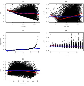
Figure 2: Several regression diagnostics plots for the CPS1988 dataset.
Chapter 13 (Regression: Troubleshooting)
R Lab
See theR scriptRlab.R for this chapter. To make the plots more visible I had to change the
y limits of the suggested plots. When these limits are changed we get the sequence of plots
shown in Figure 2. The plots (in the order in which they are coded to plot) are given by
• The externally studentized residuals as a function of the fitted values which is used to
look for heteroscedasticity (non constant variance).
• The absolute value of the externally studentized residuals as a function of the fitted values which is used to look for heteroscedasticity.
• The qqplot is used to look for error distributions that are skewed or significantly
non-normal. This might suggest applying a log or square root transformation to the
• Plots of the externally studentized residuals as a function of the variable education
which can be used to look for nonlinear regression affects in the given variable.
• Plots of the externally studentized residuals as a function of the variable experience
which can be used to look for nonlinear regression affects in the given variable.
There are a couple of things of note from this plot. The most striking item in the plots presented is in the qqplot. The right limit of the qqplot has a large deviation from a streight line. This indicates that the residuals are not normally distributed and perhaps a transformation of the response will correct this.
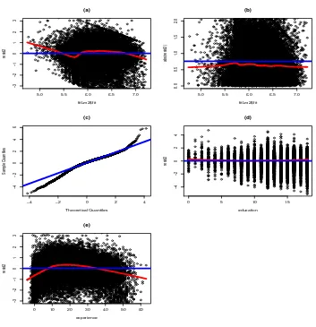
We choose to apply a log transformation to the response wage and not to use ethnicity
as a predictor (as was done in the previous part of this problem). When we plot the same diagnostic plots as earlier (under this new model) we get the plots shown in Figure 3. The qqplot in this case looks “more” normal (at least both tails of the residual distribution are more symmetric). The distribution of residuals still has heavy tails but certainly not as severe as they were before (without the log transformation). After looking at the plots in Figure 3 we see that there are still non-normal residuals. We also see that it looks like there
is a small nonlinear affect in the variable experience. We could fit a model that includes
this term. We can try a model of log(wage) with a quadratic term. When we do that, and
then reconsider the diagnostic plots presented so far we get the plots shown in Figure 4.
We can then add in the variable ethnicity and reproduce the same plots be have been
presenting previously. These plots look much like the last ones presented.
Exercises
Exercise 13.1
Some notes on the diagnostic plots are
• From Plot (a) there should be a nonlinear term in x added to the regression.
• From Plot (b) we have some heteroscedasticity in that it looks like we have different
values of variance for small and larger values of ˆy.
• From Plot (c) there might be some heavy tails and or some outliers.
• From Plot (d) it looks like we have autocorrelated errors.
5.0 5.5 6.0 6.5 7.0
−3
−2
−1
0
1
2
3
(a)
fitLm2$fit
resid2
5.0 5.5 6.0 6.5 7.0
0.0
0.5
1.0
1.5
2.0
(b)
fitLm2$fit
abs(resid2)
−4 −2 0 2 4
−4
−2
0
2
4
6
(c)
Theoretical Quantiles
Sample Quantiles
0 5 10 15
−4
−2
0
2
4
(d)
education
resid2
0 10 20 30 40 50 60
−3
−2
−1
0
1
2
3
(e)
experience
resid2
Figure 3: Several regression diagnostic plots for the CPS1988 dataset where we apply a log
4.0 4.5 5.0 5.5 6.0 6.5 7.0
−3
−2
−1
0
1
2
3
(a)
fitLm3$fit
resid3
4.0 4.5 5.0 5.5 6.0 6.5 7.0
0.0
0.5
1.0
1.5
2.0
(b)
fitLm3$fit
abs(resid3)
−4 −2 0 2 4
−4
−2
0
2
4
6
8
(c)
Theoretical Quantiles
Sample Quantiles
0 5 10 15
−4
−2
0
2
4
(d)
education
resid3
0 10 20 30 40 50 60
−3
−2
−1
0
1
2
3
(e)
experience
resid3
Figure 4: Several regression diagnostic plots for the CPS1988 dataset where we apply a log
transformation to the response and model with a quadratic term in experience (as well as
Exercise 13.2
Most of these plots seem to emphasis an outlier (the sample with index 58). This sample should be investigated and most likely removed.
Exercise 13.3
Some notes on the diagnostic plots are
• From Plot (a) there should be a nonlinear term in x added to the regression.
• From Plot (b) we don’t have much heteroscedasticity i.e. the residual variance looks
uniform.
• From Plot (d) it looks like we have autocorrelated residual errors.
Exercise 13.4
Some notes on the diagnostic plots are
• From Plot (a) there is perhaps a small nonlinear term in xthat could be added to the
regression.
• From Plot (c) we see that the distribution of the residuals have very large tails. Thus
we might want to consider taking a logarithmic or a square root transformation of the
response Y.
Chapter 14 (Regression: Advanced Topics)
Notes on the Text
The maximum likelihood estimation of σ2
To evaluate what σ is once β has been computed, we take the derivative of LGAUSS with
respect to σ, set the result equal to zero, and then solve for the value of σ. For the first
derivative ofLGAUSS we have
∂LGAUSS
Setting this expression equal to zero (and multiply by σ) we get
n− 1
Solving for σ then gives
σ2 = 1
Notes on the best linear prediction
If we desire to estimate Y with the linear combination β0+β1X then to compute β0 and β1
we seek to minimize E((Y −(β0−β1X))2). This can be expanded to produce a polynomial
in these two variables as
E((Y −(β0−β1X))2) =E(Y2−2Y(β0+β1X) + (β0+β1X)2)
=E(Y2−2β0Y −2β1XY +β02+ 2β0β1X+β21X2)
=E(Y2)−2β0E(Y)−2β1E(XY) +β02+ 2β0β1E(X) +β12E(X 2
). (8)
Take the β0 and β1 derivatives of this result, and then setting them equal to zero gives
0 =−2E(Y) + 2β0+ 2β1E(X) (9)
0 =−2E(XY) + 2β0E(X) + 2β1E(X2), (10)
as the two equations we must solve forβ0 andβ1 to evaluate the minimum of our expectation.
Writing the above system in matrix notation gives
Using Cramer’s rule we find
Thus we see that
β1 =
From Equation 9 we have
β0 =E(Y)−β1E(X) =E(Y)−
These are the equations presented in the text.
Notes on the error of the best linear prediction
Once we have specified β0 and β1 we can evaluate the expected error in using these values
for our parameters. With ˆY = ˆβ0 + ˆβ1X and the expressions we computed for β0 and β1
when we use Equation 8 we have
Since σXY =σXσYρXY we can write the above as
E((Y −Yˆ)2) =σY2 1−ρ2XY
, (13)
which is the equation presented in the book. Next we evaluate the expectation of (Y −c)2
for a constant c. We find
E((Y −c)2) =E((Y −E(Y) +E(Y)−c)2)
=E((Y −E(Y))2
+ 2(Y −E(Y))(E(Y)−c) + (E(Y)−c)2
)
=E((Y −E(Y))2
) + 0 +E((E(Y)−c)2
))
= Var (Y) + (E(Y)−c)2
, (14)
since this last term is a constant (independent of the random variable Y).
R Lab
See theR scriptRlab.R for this chapter where these problems are worked.
Regression with ARMA Noise
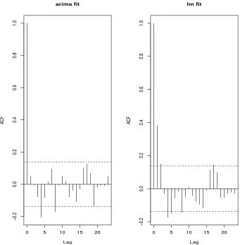
When the above R code is run it computes the two requested AIC values
[1] "AIC(arima fit)= 86.852; AIC(lm fit)= 138.882"
and also generates Figure 2. Note that both of these diagnostics indicate that the model that considers autocorrelation of residuals is the preferred model i.e. this would mean the
model computed using the R command arima. I was not exactly sure how to compute the
BIC directly but since it is related to the AIC (which the output of the arima command
gives us) I will compute it using
BIC = AIC +{log(n)−2}p .
Using this we find
[1] "BIC(arima fit)= 96.792; BIC(lm fit)= 145.509"
which again specifies that the first model is better. We can fit several ARIMA models and compare the BIC of each. When we do that we find
0 5 10 15 20
−0.2
0.0
0.2
0.4
0.6
0.8
1.0
Lag
ACF
arima fit
0 5 10 15 20
−0.2
0.0
0.2
0.4
0.6
0.8
1.0
Lag
ACF
lm fit
Figure 5: Left: Autocorrelation function for the residuals for thearimafit of theMacroDiff
dataset. Right: Autocorrelation function for the residuals for the lm fit of the MacroDiff
(a)
Time
r1
1950 1960 1970 1980 1990
0
5
10
15
(b)
Time
delta_r1
1950 1960 1970 1980 1990
−4
−2
0
2
(c)
Time
delta_r1^2
1950 1960 1970 1980 1990
0
5
10
15
20
0 5 10 15
−4
−2
0
2
(d)
lag_r1
delta_r1
0 5 10 15
0
5
10
15
20
(e)
lag_r1
delta_r1^2
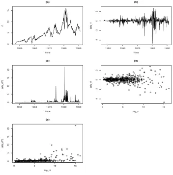
Figure 6: The plots for estimating the short rate models.
Nonlinear Regression
The R command help(Irates) tells us that the r1 column from the Irates dataframe is
a ts object of interest rates sampled each month from Dec 1946 until Feb 1991 from the
United-States. These rates are expressed as a percentage per year.
When the above R code is run we get the plots shown in Figure 6. These plots are used in
building the models forµ(t, r) and σ(t, r). From the plot labeled (d) we see that ∆rt seems
(on average) to be relatively constant at least for small values of rt−1 i.e. less than 10. For
values greater than that we have fewer samples and it is harder to say if a constant would be
the best fitting function. From the plot labeled (b) it looks like there are times when ∆rt is
larger than others (namely around 1980s). This would perhaps argue for a time dependent
µ function. There does not seem to be a strong trend. From the summary command we see
that a and θ are estimated as
Formula: delta_r1 ~ a * (theta - lag_r1)
Parameters:
Estimate Std. Error t value Pr(>|t|)
theta 5.32754 1.33971 3.977 7.96e-05 ***
a 0.01984 0.00822 2.414 0.0161 *
Response Transformations
The boxcox function returns x which is a list of the values ofα tried andy the value of the
loglikelihood for each of these values ofα. We want to pick a value ofα that maximizes the
loglikelihood. Finding the maximum of the loglikelihood we see that it is achieved at a value
of α = 0.1414141. The new model with Y transformed using the box-cox transform has a
much smaller value of the AIC
[1] "AIC(fit1)= 12094.187991, AIC(fit3)= 1583.144759"
This is a significant reduction in AIC. Plots of the residuals of the box-cox model as a function of the fitted values indicate that there is not a problem of heteroscedasticity. The residuals of this box-cox fit appear to be autocorrelated but since this is not time series data this behavior is probably spurious (not likely to repeat out of sample).
Who Owns an Air Conditioner?
Computing a linear model using all of the variables gives that several of the coefficients are
not estimated well (given the others in the model). We find
> summary(fit1)
Call:
glm(formula = aircon ~ ., family = "binomial", data = HousePrices)
Deviance Residuals:
Min 1Q Median 3Q Max
-2.9183 -0.7235 -0.5104 0.6578 3.2650
Coefficients:
Estimate Std. Error z value Pr(>|z|)
(Intercept) -3.576e+00 5.967e-01 -5.992 2.07e-09 ***
price 5.450e-05 8.011e-06 6.803 1.02e-11 ***
lotsize -4.482e-05 6.232e-05 -0.719 0.472060
bathrooms -5.587e-01 2.705e-01 -2.065 0.038907 *
stories 3.155e-01 1.540e-01 2.048 0.040520 *
drivewayyes -4.089e-01 3.550e-01 -1.152 0.249366
recreationyes 1.052e-01 2.967e-01 0.355 0.722905
fullbaseyes 1.777e-02 2.608e-01 0.068 0.945675
gasheatyes -3.929e+00 1.121e+00 -3.506 0.000454 ***
garage 6.893e-02 1.374e-01 0.502 0.615841
preferyes -3.294e-01 2.743e-01 -1.201 0.229886
We can use the stepAIC in the MASS library to sequentially remove predictors. The final
step from the stepAIC command gives
Step: AIC=539.36
aircon ~ price + bathrooms + stories + gasheat
Df Deviance AIC
<none> 529.36 539.36
- bathrooms 1 532.87 540.87
- stories 1 535.46 543.46
- gasheat 1 554.74 562.74
- price 1 615.25 623.25
The summary command on the resulting linear model gives
> summary(fit2)
Call:
glm(formula = aircon ~ price + bathrooms + stories + gasheat, family = "binomial", data = HousePrices)
Deviance Residuals:
Min 1Q Median 3Q Max
-2.8433 -0.7278 -0.5121 0.6876 3.0753
Coefficients:
Estimate Std. Error z value Pr(>|z|)
(Intercept) -4.045e+00 4.050e-01 -9.987 < 2e-16 ***
price 4.782e-05 6.008e-06 7.959 1.73e-15 ***
bathrooms -4.723e-01 2.576e-01 -1.833 0.066786 .
stories 3.224e-01 1.317e-01 2.449 0.014334 *
gasheatyes -3.657e+00 1.082e+00 -3.378 0.000729 ***
table, increasing bathrooms and gasheatyes should decrease the probability that we have air conditioning. One would not expect that having more bathrooms should decrease our
probability of air conditioning. The same might be said for the gasheatyes predictor. The
difference in AIC between the model suggested and the one when we remove the predictor
bathroomsis not very large indicating that removing it does not give a very different model. As the sample we are told to look at seems to be the same as the first element in the training
set we can just extract that sample and use the predict function to evaluate the given
model. When we do this (using the first model) we get 0.1191283.
Exercises
Exercise 14.1 (computing β0 and β1)
See the notes on Page 14.
Exercise 14.2 (hedging)
The combined portfolio is
F20P20−F10P10−F30P30.
Lets now consider how this portfolio changes as the yield curve changes. From the book we would have that the change in the total portfolio is given by
−F20P20DUR20∆y20+F10P10DUR10∆y10+F30P30DUR30∆y30.
We are told that we have modeled ∆y20 as
∆y20= ˆβ1∆y10+ ˆβ2∆y30.
When we put this expression for ∆y20 into the above (and then group by ∆y10 and ∆y30)
we can write the above as
(−F20P20DUR20βˆ1 +F10P10DUR10)∆y10+ (−F20P20DUR20βˆ2+F30P30DUR30)∆y30.
We will then take F10 and F30 to be the values that would make the coefficients of ∆y10 and
∆y30 both zero. These would be
F10 =F20
P20DUR20
P10DUR10
ˆ
β1
F30=F20
P20DUR20
P30DUR30
ˆ
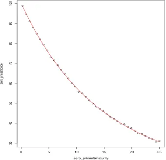
Exercise 14.3 (fitting a yield curve)
We are given the short rater(t;θ), which we need to integrate to get the yield yt(θ). For the
Nelson-Siegel model for r(t;θ) this integration is presented in the book on page 383. Then
given the yield the price is given by
Pi = exp(−TiyTi(θ)) +ǫi.
I found it hard to fit the model “all at once”. In order to fit the model I had to estimate
each parameter θi in a sequential fashion. See theR codechap 14.Rfor the fitting procedure
used. When that code is run we get estimate of the four θ parameters given by
theta0 theta1 theta2 theta3
0.009863576 0.049477242 0.002103376 0.056459908
0 5 10 15 20 25
30
40
50
60
70
80
90
100
zero_prices$maturity
zero_pr
ices$pr
ice
Chapter 17 (Factor Models and Principal Components)
Notes on the Book
Notes on Estimating Expectations and Covariances using Factors
Given the expression for Rj,t we can evaluate the covariance between two difference asset
returns as follows
Cov (Rj,t, Rj′,t) = Cov (β0,j+β1,jF1,t+β2,jF2,t+ǫj,t, β0,j′ +β1,j′F1,t+β2,j′F2,t+ǫj′,t) = Cov (β1,jF1,t, β0,j′ +β1,j′F1,t+β2,j′F2,t+ǫj′,t)
+ Cov (β2,jF2,t, β0,j′ +β1,j′F1,t+β2,j′F2,t+ǫj′,t) + Cov (ǫj,t, β0,j′ +β1,j′F1,t+β2,j′F2,t+ǫj′,t) =β1,jβ1,j′Var (F1,t) +β1,jβ2,j′Cov (F1,t, F2,t)
+β2,jβ1,j′Cov (F2,t, F1,t) +β2,jβ2,j′Var (F2,t)
=β1,jβ1,j′Var (F1,t) +β2,jβ2,j′Var (F2,t) + (β1,jβ2,j′+β1,j′β2,j)Cov (F1,t, F2,t) ,
which is the same as the books equation 17.6.
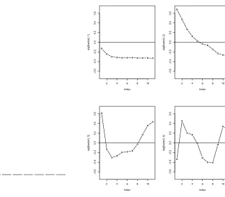
R Lab
See the R script Rlab.R for this chapter. We first duplicate the bar plot of the eigenvalues
and eigenvectors of the covariance matrix of the dataframe yielddat. These are shown in
Figure 8.
Problem 1-2 (for fixed maturity are the yields stationary?)
See Figure 9 for a plot of the first four columns of the yield data (the first four maturities). These plots do not look stationary. This is especially true for index values from 1000 to 1400 where all yield curves seem to trend upwards.
As suggested in the book we can also use the augmented Dickey-Fuller test to test for stationarity. When we do this for each possible maturity we get
0.0
Figure 8: Left: The distribution of the eigenvalues of the yield data. Right: Plots of the
first four eigenvectors of the yield data.
[1] "column index= 6; p_value= 0.386320" [1] "column index= 7; p_value= 0.391729" [1] "column index= 8; p_value= 0.437045" [1] "column index= 9; p_value= 0.461692" [1] "column index= 10; p_value= 0.460651" [1] "column index= 11; p_value= 0.486028"
As all of these p values are “large” (none of them are less than 0.05) we can conclude that
the raw yield curve data is notstationary.
Problem 3 (for fixed maturity are the difference in yields stationary?)
See Figure 10 for a plot of the first difference of each of the four columns of the yield data
(the first difference of the first four maturities). These plots now dolook stationary. Using
the augmented Dickey-Fuller test we can show that the time series of yield differences are stationarity. Using the same code as before we get
0 200 400 600 800 1000 1400
4
5
6
7
8
Index
yieldDat[, 1]
0 200 400 600 800 1000 1400
4
5
6
7
8
Index
yieldDat[, 2]
0 200 400 600 800 1000 1400
4
5
6
7
8
Index
yieldDat[, 3]
0 200 400 600 800 1000 1400
4
5
6
7
8
Index
yieldDat[, 4]
0 200 400 600 800 1000 1400
−0.4
−0.2
0.0
0.2
0.4
0.6
Index
delta_yield[, 1]
0 200 400 600 800 1000 1400
−0.3
−0.2
−0.1
0.0
0.1
0.2
Index
delta_yield[, 2]
0 200 400 600 800 1000 1400
−0.3
−0.2
−0.1
0.0
0.1
0.2
0.3
Index
delta_yield[, 3]
0 200 400 600 800 1000 1400
−0.3
−0.2
−0.1
0.0
0.1
0.2
0.3
Index
delta_yield[, 4]
[1] "column index= 3; p_value= 0.010000" [1] "column index= 4; p_value= 0.010000" [1] "column index= 5; p_value= 0.010000" [1] "column index= 6; p_value= 0.010000" [1] "column index= 7; p_value= 0.010000" [1] "column index= 8; p_value= 0.010000" [1] "column index= 9; p_value= 0.010000" [1] "column index= 10; p_value= 0.010000" [1] "column index= 11; p_value= 0.010000"
There were 11 warnings (use warnings() to see them)
As all of these p values are “small” (they are all less than 0.01) we can conclude that the
first differences of a yield at a fixed maturity is stationary. The warnings indicates that
the adf.test command could not actually compute the correct p-value and that the true
p-values are actually smaller than the ones printed above.
Problem 4 (PCA on differences between the yield curves)
Part (a): The variable sdev holds the standard deviations of each principal components,
these are also the square root of the eigenvalues of the covariance matrix. The variable
loadings hold the eigenvectors of the covariance matrix. The variable center hold the means that were subtracted in each feature dimension in computing the covariance matrix.
The variable scores holds a matrix of each vector variable projected into all its principle
components. We can check that this is so by comparing the two outputs
t(as.matrix(pca_del$loadings[,])) %*% t( delta_yield[1,] - pca_del$center ) 2
Comp.1 0.1905643953
Comp.2 0.0375662026
Comp.3 0.0438591813
Comp.4 -0.0179855611
Comp.5 0.0002473111
Comp.6 0.0002924385
Comp.7 0.0101975886
Comp.8 -0.0093768514
Comp.9 -0.0036798653
Comp.10 0.0004287954
Comp.11 -0.0005602180
with
0.1905643953 0.0375662026 0.0438591813 -0.0179855611 0.0002473111
Comp.6 Comp.7 Comp.8 Comp.9 Comp.10
0.0002924385 0.0101975886 -0.0093768514 -0.0036798653 0.0004287954
Comp.11 -0.0005602180
These two outputs are exactly the same (as they should be).
Part (b): Squaring the first two values of the sdev output we get
> pca_del$sdev[1:2]^2
Comp.1 Comp.2
0.031287874 0.002844532
Part (c): The eigenvector corresponding to the largest eigenvalue is the first one and has
values given by
> pca_del$loadings[,1]
X1mon X2mon X3mon X4mon X5mon X5.5mon
-0.06464327 -0.21518811 -0.29722014 -0.32199492 -0.33497517 -0.33411403
X6.5mon X7.5mon X8.5mon X9.5mon NA.
-0.33220277 -0.33383143 -0.32985565 -0.32056039 -0.31668346
Part (d): Using the output from thesummary(pca_del)which in a truncated form is given
by
Importance of components:
Comp.1 Comp.2 Comp.3 Comp.4 Comp.5
Standard deviation 0.1768838 0.05333415 0.03200475 0.014442572 0.011029556
Proportion of Variance 0.8762330 0.07966257 0.02868616 0.005841611 0.003406902
Cumulative Proportion 0.8762330 0.95589559 0.98458175 0.990423362 0.993830264
we see from the Cumulative Proportion row above that to obtain 95% of the variance we
must have at least 2 components. Taking three components gives more than 98% of the variance.
Problem 5 (zero intercepts in CAPM?)
The output of the lm gives the fitted coefficients and their standard errors, capturing the
Response GM :
Estimate Std. Error t value Pr(>|t|)
(Intercept) -0.0103747 0.0008924 -11.626 <2e-16 ***
FF_data$Mkt.RF 0.0124748 0.0013140 9.494 <2e-16 ***
Response Ford :
Estimate Std. Error t value Pr(>|t|)
(Intercept) -0.0099192 0.0007054 -14.06 <2e-16 ***
FF_data$Mkt.RF 0.0131701 0.0010386 12.68 <2e-16 ***
Response UTX :
Estimate Std. Error t value Pr(>|t|)
(Intercept) -0.0080626 0.0004199 -19.20 <2e-16 ***
FF_data$Mkt.RF 0.0091681 0.0006183 14.83 <2e-16 ***
Response Merck :
Estimate Std. Error t value Pr(>|t|)
(Intercept) -0.0089728 0.0009305 -9.643 < 2e-16 ***
FF_data$Mkt.RF 0.0062294 0.0013702 4.546 6.85e-06 ***
Notice that the p-value of all intercepts are smaller than the given value of α i.e. 5%. Thus
we cannotaccept the hypothesis that the coefficient β0 is zero.
Problem 6
We can use the cor command to compute the correlation of the residuals of each of the
CAPM models which gives
> cor( fit1$residuals )
GM Ford UTX Merck
GM 1.00000000 0.55410840 0.09020925 -0.04331890
Ford 0.55410840 1.00000000 0.09110409 0.03647845
UTX 0.09020925 0.09110409 1.00000000 0.05171316
Merck -0.04331890 0.03647845 0.05171316 1.00000000
The correlation between GM and Ford is quite large. To get confidence intervals for each
correlation coefficient we will use the command cor.test to compute the 95% confidence
intervals. We find
[1] "Correlation between Ford and GM; ( 0.490439, 0.554108, 0.611894)"
[1] "Correlation between UTX and GM; ( 0.002803, 0.090209, 0.176248)"
[1] "Correlation between Merck and Ford; ( -0.051113, 0.036478, 0.123513)"
[1] "Correlation between Merck and UTX; ( -0.035878, 0.051713, 0.138515)"
From the above output only the correlations between Merck and GM, Ford, and UTX seem to be zero. The others don’t seem to be zero.
Problem 7 (comparing covariances)
The sample covariance or ΣR can be given by using the cov command. Using the factor
returns the covariance matrix ΣR can be written as
ΣR=βTΣFβ+ Σǫ, (15)
whereβis therowvector of each stocks CAPM beta value. In theRcodeRlab.Rwe compute
both ΣR and the right-hand-side of Equation 16 (which we denote as ˆΣ). If we plot these
two matrices sequentially we get the following
> Sigma_R
GM Ford UTX Merck
GM 4.705901e-04 2.504410e-04 6.966363e-05 1.781501e-05
Ford 2.504410e-04 3.291703e-04 6.918793e-05 4.982034e-05
UTX 6.966363e-05 6.918793e-05 1.270578e-04 3.645322e-05
Merck 1.781501e-05 4.982034e-05 3.645322e-05 4.515822e-04 > Sigma_R_hat
GM Ford UTX Merck
GM 4.705901e-04 7.575403e-05 5.273459e-05 3.583123e-05
Ford 7.575403e-05 3.291703e-04 5.567370e-05 3.782825e-05
UTX 5.273459e-05 5.567370e-05 1.270578e-04 2.633334e-05
Merck 3.583123e-05 3.782825e-05 2.633334e-05 4.515822e-04
The errors between these two matrices are primarily in the off diagonal elements. We expect the pairs that have their residual correlation non-zero to have the largest discrepancy. If we consider the absolute value of the difference of these two matrices we get
> abs( Sigma_R - Sigma_R_hat )
GM Ford UTX Merck
GM 1.084202e-19 1.746870e-04 1.692904e-05 1.801622e-05
Ford 1.746870e-04 2.168404e-19 1.351424e-05 1.199209e-05
UTX 1.692904e-05 1.351424e-05 1.084202e-19 1.011988e-05
Merck 1.801622e-05 1.199209e-05 1.011988e-05 0.000000e+00
Problem 8 (the beta of SMB and HML)
If we look at the p-values of the fitted model on each stock we are getting results like the
following
> sfit2$’Response GM’$coefficients
Estimate Std. Error t value Pr(>|t|) (Intercept) -0.010607689 0.000892357 -11.887271 7.243666e-29 FF_data$Mkt.RF 0.013862140 0.001565213 8.856390 1.451297e-17 FF_data$SMB -0.002425130 0.002308093 -1.050708 2.939015e-01 FF_data$HML 0.006373645 0.002727395 2.336899 1.983913e-02 > sfit2$’Response GM’$coefficients
Estimate Std. Error t value Pr(>|t|) (Intercept) -0.010607689 0.000892357 -11.887271 7.243666e-29 FF_data$Mkt.RF 0.013862140 0.001565213 8.856390 1.451297e-17 FF_data$SMB -0.002425130 0.002308093 -1.050708 2.939015e-01 FF_data$HML 0.006373645 0.002727395 2.336899 1.983913e-02 > sfit2$’Response Ford’$coefficients
Estimate Std. Error t value Pr(>|t|)
(Intercept) -1.004705e-02 0.0007082909 -14.18492403 1.296101e-38 FF_data$Mkt.RF 1.348451e-02 0.0012423574 10.85396920 8.752040e-25 FF_data$SMB -7.779018e-05 0.0018320033 -0.04246181 9.661475e-01 FF_data$HML 3.780222e-03 0.0021648160 1.74620926 8.138996e-02 > sfit2$’Response UTX’$coefficients
Estimate Std. Error t value Pr(>|t|) (Intercept) -0.0080963376 0.0004199014 -19.2815220 2.544599e-62 FF_data$Mkt.RF 0.0102591816 0.0007365160 13.9293389 1.721546e-37 FF_data$SMB -0.0028475161 0.0010860802 -2.6218286 9.013048e-03 FF_data$HML 0.0003584478 0.0012833841 0.2792989 7.801311e-01 > sfit2$’Response Merck’$coefficients
Estimate Std. Error t value Pr(>|t|) (Intercept) -0.008694614 0.000926005 -9.389381 2.142386e-19 FF_data$Mkt.RF 0.007065701 0.001624233 4.350178 1.650293e-05 FF_data$SMB -0.004094797 0.002395124 -1.709639 8.795427e-02 FF_data$HML -0.009191144 0.002830236 -3.247483 1.242661e-03
In the fits above we see that the slope of the SMB and HML for different stocks have significance at the 2% - 8% level. For example, the HML slope for GM is significant at the 1.9% level. Based on this we cannot accept the null hypothesis of zero value for slopes.
Problem 9 (correlation of the residuals in the Fama-French model)
If we look at the 95% confidence interval under the Fama-French model we get
[1] "Correlation between Ford and GM; ( 0.487024, 0.550991, 0.609079)"
[1] "Correlation between UTX and GM; ( -0.004525, 0.082936, 0.169138)"
[1] "Correlation between UTX and Ford; ( 0.002240, 0.089651, 0.175702)"
[1] "Correlation between Merck and UTX; ( -0.040087, 0.047508, 0.134378)"
Now the correlation between UTX and GM is zero (it was not in the CAPM). We still have a significant correlation between Ford and GM and between UTX and Ford (but it is now smaller).
Problem 10 (model fitting)
The AIC and BIC between the two models is given by
[1] "AIC(fit1)= -10659.895869; AIC(fit2)= -10688.779045" [1] "BIC(fit1)= -10651.454689; BIC(fit2)= -10671.896684"
The smaller value in each case comes from the second fit or the Fama-French model.
Problem 11 (matching covariance)
The two covariance matrices are now
> Sigma_R
GM Ford UTX Merck
GM 4.705901e-04 2.504410e-04 6.966363e-05 1.781501e-05
Ford 2.504410e-04 3.291703e-04 6.918793e-05 4.982034e-05
UTX 6.966363e-05 6.918793e-05 1.270578e-04 3.645322e-05
Merck 1.781501e-05 4.982034e-05 3.645322e-05 4.515822e-04 > Sigma_R_hat
GM Ford UTX Merck
GM 4.705901e-04 7.853015e-05 5.432317e-05 3.108052e-05
Ford 7.853015e-05 3.291703e-04 5.602592e-05 3.437406e-05
UTX 5.432317e-05 5.602592e-05 1.270578e-04 2.733456e-05
Merck 3.108052e-05 3.437406e-05 2.733456e-05 4.515822e-04
The difference between these two matrices are smaller than in the CAPM model.
Problem 12 (Fama-French betas to excess returns covariance)
We will use the formula
ΣR=βTΣFβj+ Σǫ. (16)
Mkt.RF SMB HML
Mkt.RF 0.46108683 0.17229574 -0.03480511
SMB 0.17229574 0.21464312 -0.02904749
HML -0.03480511 -0.02904749 0.11023817
This factor covariance matrix will not change if the stock we are considering changes.
Part (a-c): Given the factor loadings for each of the two stocks and their residual variances
we can compute the right-hand-side of Equation 16 and find
[,1] [,2]
[1,] 23.2254396 0.1799701
[2,] 0.1799701 37.2205144
Thus we compute that the variance of the excess return of Stock 1 is 23.2254396, the variance of the excess return of Stock 2 is 37.2205144 and the covariance between the excess return of Stock 1 and Stock 2 is 0.1799701.
Problem 13
Using the factanal command we see that the factor loadings are given by
Factor1 Factor2
GM_AC 0.874 -0.298
F_AC 0.811
UTX_AC 0.617 0.158
CAT_AC 0.719 0.286
MRK_AC 0.719 0.302
PFE_AC 0.728 0.208
IBM_AC 0.854
MSFT_AC 0.646 0.142
The variance of the unique risks for Ford and GM are the values that are found in the “Uniquenesses” list which we found is given by
GM_AC F_AC UTX_AC CAT_AC MRK_AC PFE_AC IBM_AC MSFT_AC
0.148 0.341 0.594 0.401 0.392 0.427 0.269 0.562
Problem 14
The p-value for the factanal command is very small 1.39 10−64 indicating that we should
reject the null hypothesis and try a larger number of factors. Using four factors (the largest
that we can use with eight inputs) gives a larger p-value 0.00153.
Problem 15
For statistical factor models the covariance between the log returns is given by
ΣR = ˆβTβˆ+ ˆΣǫ,
where the ˆβ and ˆΣǫ are the estimated loadings and uniqueness found using the factanal
command. When we do that we get an approximate value for ΣR given by
[,1] [,2] [,3] [,4] [,5] [,6] [,7] [,8]
[1,] 1.0000002 0.6944136 0.4920453 0.5431030 0.5381280 0.5737600 0.7556789 0.5223550 [2,] 0.6944136 1.0000012 0.5075905 0.5961289 0.5966529 0.5994766 0.6909546 0.5305168 [3,] 0.4920453 0.5075905 0.9999929 0.4892064 0.4915723 0.4821511 0.5222193 0.4215048 [4,] 0.5431030 0.5961289 0.4892064 0.9999983 0.6034673 0.5829600 0.6052811 0.5055927 [5,] 0.5381280 0.5966529 0.4915723 0.6034673 1.0000019 0.5860924 0.6045542 0.5076939 [6,] 0.5737600 0.5994766 0.4821511 0.5829600 0.5860924 1.0000006 0.6150548 0.5000431 [7,] 0.7556789 0.6909546 0.5222193 0.6052811 0.6045542 0.6150548 1.0000003 0.5476733 [8,] 0.5223550 0.5305168 0.4215048 0.5055927 0.5076939 0.5000431 0.5476733 0.9999965
As Ford is located at index 2 and IBM is located at index 7 we want to look at the (2,7)th
or (7,2)th element of the above matrix where we find the value 0.6909546.
Exercises
Exercise 17.1-2
These are very similar to the Rlab for this chapter.
Exercise 17.3
Chapter 21 (Nonparametric Regression and Splines)
Notes on the Text
Notes on polynomial splines
When we force the linear fits on each side of the knot x=t to be continuous we have that
a+bt = c+dt and this gives c =a+ (b−d)t. When we use this fact we can simplify the
formula for s(x) when x > t as
s(x) =c+dx=a+ (b−d)t+dx
=a+bt+d(x−t) =a+bx−bx+bt+d(x−t)
=a+bx−b(x−t) +d(x−t) =a+bx+ (d−b)(x−t),
which is the books equation 21.11.
R Lab
See theR scriptRlab.R for this chapter.
R lab: An Additive Model for Wages, Education, and Experience
When we enter and then run the givenR code we see that thesummary command gives that
β0 = 6.189742 and β1 =−0.241280.
Plots from the fitGam are duplicated in Figure 11.
R lab: An Extended CKLS model for the Short Rate
We are using 10 knots. The outerfunction here takes the outer difference of the values in t
with those in knots. The statement that computes X2then computes the value of the “plus”
functions for the various knots i.e. evaluates (t−k)+ where t is the time variable and k is
a knot. Then X3 holds the linear spline basis function i.e. the total spline we are using to
predict µ(t, r) is given by
α0+α1t+ 10
X
i=1
θi(t−ki)+.
0
5
10
15
−2.0 −1.5 −1.0 −0.5 0.0 0.5 1.0
education
s(education,7.65)
0
10
20
30
40
50
60
−2.0 −1.5 −1.0 −0.5 0.0 0.5 1.0
e
xper
ience
s(experience,8.91)
F
ig
u
re
11
:
P
lo
ts
fo
r
th
e
sp
lin
es
C
P
S
1
9
8
8
d
at
as
et
.
1950 1960 1970 1980 1990
0
5
10
15
(a)
t
rate
theta(t) lagged rate
1950 1960 1970 1980 1990
0.08
0.10
0.12
0.14
0.16
0.18
(b)
t
a(t)
0 5 10 15
0
1
2
3
4
5
6
(c)
lag_r1 abs res volatility fn
Figure 12: The three plots for the short rate example.
the constant α0 term), the second column of X3 is a column of time relative to 1946. The
rest of the columns of X3 are samples of the spline basis “plus” functions i.e. (t−ki)+ for
1≤i≤10. When we run the givenR code we generate the plot in Figure 12. Note that
X3[,1:2]%*%a
is a linear function in t but because of the way that X3 is constructed (its last 10 columns)
X3%*%theta
is the evaluation of a spline. Our estimates of the coefficients ofα0andα1are not significant.
A call to summary( nlmod_CKLS_ext )$parameters gives
Estimate Std. Error t value Pr(>|t|)
The large p-values indicate that these coefficients are not well approximated and might not be real effects.
Exercises
Exercise 21.1 (manipulations with splines)
Our expression fors(t) is given by
s(t) =β0 +β1x+b1(x−1)++b2(x−2)++b3(x−3)+.
Where the “plus function” is defined by
(x−t)+ =
0 x < t x−t x≥t
From the given values ofx and s(x) we can compute
s(0) = 1 =β0
s(1) = 1.3 = 1 +β1 so β1 = 0.3
s(2) = 5.5 = 1 + 0.3(2) +b1(1) so b1 = 3.9
s(4) = 6 = 1 + 0.3(4) + 3.9(3) +b2(2) +b3(1)
s(5) = 6 = 1 + 0.3(5) + 3.9(4) +b2(3) +b3(2).
Solving these two equations gives b2 =−3.7 and b3 =−0.5. Thus we have s(x) given by
s(x) = 1 + 0.3x+ 3.9(x−1)+−3.7(x−2)+−0.5(x−3)+.
Part (a): We would find
s(0.5) = 1 + 0.3(0.5) = 1.15.
Part (b): We would find
s(3) = 1 + 0.3(3) + 3.9(2)−3.7(1) = 6.
Part (c): We would evaluate
Z 4
2
s(t)dt=
Z 4
2
(1 + 0.3t+ 3.9(t−1)−3.7(t−2))dt−0.5
Z 4
3
(t−3)dt ,
Exercise 21.2
The model 21.1 in the book is
∆rt=rt−rt−1 =µ(rt−1) +σ(rt−1)ǫt. (17)
In this problem we are told functional forms forµ(rt−1) and σ(rt−1).
Part (a): Since ǫt has a mean of zero we have that
E[rt|rt−1 = 0.04] =rt−1+µ(rt−1) = 0.04 + 0.1(0.035−0.04) = 0.0395.
Part (b): Since ǫt has a variance of one we have that
Var (rt|rt−1 = 0.02) =σ2(rt−1) = 2.32rt−12 = 2.32(0.02)2 = 0.002116.
Exercise 21.4
For the given spline we have
s′
(x) = 0.65 + 2x+ 2(x−1)++ 1.2(x−2)+
s′′
(x) = 2 + 2(x−1)0
++ 1.2(x−1.2) 0 +.
Part (a): We have
s(1.5) = 1 + 0.65(1.5) + 1.52+ 0.52 = 4.475.
and
s′
(1.5) = 0.65 + 3 + 2(0.5) + 1.2(0) = 4.65.
Part (b): We have
s′′