*Corresponding author. Tel.:#44-0171-955-7509; fax:#44-0171-831-1840. E-mail address:[email protected] (P.M. Robinson).
The memory of stochastic volatility models
P.M. Robinson
*
Department of Economics, London School of Economics, Houghton Street, London WC2A 2AE, UK
Received 17 February 1999; received in revised form 28 July 2000; accepted 1 August 2000
Abstract
A valid asymptotic expansion for the covariance of functions of multivariate normal vectors is applied to approximate autocovariances of time series generated by nonlinear transformation of Gaussian latent variates, and nonlinear functions of these, with special reference to long memory stochastic volatility models, serving to identify the roles played by the underlying Gaussian processes and the nonlinear transformation. Implications for simple stochastic volatility models are examined in detail, with numerical and Monte Carlo calculations, and applications to cyclic behaviour, cross-sectional and temporal aggregation, and multivariate models are discussed. ( 2001 Elsevier Science S.A. All rights reserved.
JEL classixcation: C22
Keywords: Stochastic volatility; Long memory; Nonlinear functions of Gaussian pro-cesses
1. Introduction
A major theme of nonlinear time-series analysis in"nance and econometrics concerns the in#uence of instantaneous nonlinear transformation on measures of memory. One class of measures which has featured frequently in asymptotic theory for time-series statistics is mixing numbers, which are known to be
essentially invariant to such transformation (see e.g. Ibragimov and Linnik, 1971) in the sense that their rate of decay is unchanged. However, mixing numbers cannot properly be estimated from data, and some empirical evidence about measures that can be estimated prompts further theoretical investigation.
For stationary time series the measures of this type that come most immedi-ately to mind are autocovariances (and autocorrelations, which decay at the same rate). In particular, a well-established empirical "nding is that "nancial time series levels x
t, such as daily asset returns, are apt to exhibit little or no
autocorrelation, whereas, their squares x2
t have noticeable autocorrelation.
Attempts to model this phenomenon began with the ARCH(p) model of Engle (1982), followed by its GARCH(p,q) extension (Bollerslev, 1986), and the stochastic volatility model of Taylor (1986), with numerous elaborations on these themes.
The model of Engle (1982), and the bulk of its successors, have the property thatCov(x
t, xt`j)"0, for all nonzeroj, whereasCov(x2t,x2t`j) decays
exponenti-ally to zero asjPR. Linear processes are incapable of describing this phenom-enon, but, mathematically speaking, this divergence in the properties of the levels and squares is not dramatic, and relatively recent empirical studies (see e.g. Ding et al., 1993; Granger and Ding, 1995; Ding and Granger, 1996; Andersen and Bollerslev, 1997) suggest a degree of persistence in Cov(x2
t,x2t`j), which
might be modelled in terms of a much slower rate of decay.
In fact models had already been proposed that might explain this behaviour. Robinson (1991) considered extensions of the ARCH(p) and GARCH(p, q) that might entail arbitarily slow decay of autocorrelations of x2t, including long memory, where autocorrelations are not summable, and Whistler (1990) applied relevant tests he developed to "nancial data. Ding and Granger (1996) and others have developed such models further. On the other hand, Andersen and Bollerslev (1997), Breidt et al. (1998), Harvey (1998) considered a long-memory version of Taylor's (1986) stochastic volatility model, Robinson and Za!aroni (1998) considered an alternative&2-shock'functional form, Robinson and Zaf-faroni (1997) considered a nonlinear moving average whose squares have long memory, while Teyssiere (1998) has discussed a variety of ARCH type long memory functional forms involving various forms of nonlinearity.
At the same time, other empirical"ndings must be borne in mind. A body of opinion asserts that fourth moments of many "nancial series are in"nite, in which case autocovariances of x2
t are not well de"ned. Partly in response,
autocovariances of other instantaneous transformations ofx
thave been studied,
such asDx
tDh, for real-valuedh(for exampleh"1), so that forh(2 the fourth
moment problem is avoided. Ding et al. (1993), Ding and Granger (1996), Granger and Ding (1995) found a tendency over a range of series for sample autocorrelations to be relatively large for speci"ch, such ash"1. Apart from the question of"niteness of moments, absolute powersDx
hard to handle in the context of the ARCH models of Engle (1982), Bollerslev (1986), Robinson (1991) whenhis not an even integer.
The present paper demonstrates that, for a wide variety of processes, the autocovariances at long lags of instantaneous nonlinear functions of a general type can be rigorously approximated su$ciently accurately to enable the pres-ence or abspres-ence of long memory in the instantaneous function to be determined from the speci"cation of the original process. As well as enabling us to thereby deal with particular, parametrically speci"ed, processes, our results help to explain empirical "ndings of long-memory stochastic volatility in terms of a general class of data-generating processes, allowing also the practitioner freedom to choose the form of nonlinear transformation in such a way as to minimize moment conditions, if desired.
A scalar observable (possibly transformed) seriesy
t will be modelled as
y
t"f(gt), (1.1)
wheregt is ap-dimensional stationary Gaussian process andf:RpPR. A par-ticular case of (1.1) that is of interest speci"esfto have separable form, such that
y
t"f1(g1t)f2(g2t), (1.2)
takingg
t"(g@1t, g@2t)@, wheregitispi]1,i"1, 2,p1#p2"p,Cov(g1t, g2t)"0
andf
i:RpiPR, i"1, 2. Ifxthas form (1.2), then so (for a newf1, f2) doesDxtDh,
for any h. Moreover, subject to "niteness of appropriate moments, if
Ef
1(g1t)"0, thenEyt"0 while if alsog1tis an iid sequence andg1tis
indepen-dent of g2
s,s(t, then Cov(yt, yt`j)"0, for all jO0, so that the classical
zero-autocovariance properties of asset returnsy
t"xt are described, whereas
when we takey
t"DxtDh, or its logarithm, thenEf1(g1t)O0 and moreover we can
then get autocorrelation.
The form (1.2) does not cover ARCH-type models (because p(R) but it covers such models as
x
t"g1tea`bg2t (1.3)
and
x
t"g1t(a#bg2t) (1.4)
withg1
t white noise (having zero mean),g2t either depending only ong1s,s(t
or being independent ofg1
s for alls,t, and yt"xt oryt"DxtDh. Model (1.3) is
a standard stochastic volatility model (Taylor, 1986), where Andersen and Bollerslev (1997), Breidt et al. (1998), Harvey (1998) took g2
t to have long
memory. Model (1.4) is in Robinson and Za!aroni (1997, 1998) with again
at long lags of certain nonlinear functions of (1.3). Our asymptotic expansion rigorously justi"es and re"nes such asymptotic formulae in a variety of settings. For parametric"tting of a particular parametric form such as (1.3) or (1.4) the autocorrelation in g
t would be parameterized, but this possibility does not
concern us here, except insofar as we have to employ a parameterization in generating Monte Carlo observations.
A wide range of models is covered by (1.2), entailing both short and long memory ing
t. We impose no smoothness onf1andf2and can choose them such
that only the second moment requirement
Ef2
i (git)(R, i"1, 2, (1.5)
is required, notwithstanding the Gaussianity ofg
t. By way of illustration, and
also partial motivation for our allowance ofp
i*2, consider
f
1(g1t)"
g(1)1t(p1!1)1@2
Mg(2)21t #2#g(p1)2
1t N1@2
, (1.6)
whereg(1j)
t is thejth element ofg1tand theg1(jt), 1)j)p1, are mutually
indepen-dent (see the remark after (2.1) below) but can have autocorrelation. Then (1.6) has at
p1~1distribution, having"nite integer moments up to degreep1!2 only,
for example when 2)p
1)5 it has in"nite fourth moment. Of course (1.6) has
mean zero so it might be substituted forg1
tin (1.3) and (1.4) (cf. Bollerslev, 1987),
whencex
tinherits its moment properties. Other random variables expressible as
functions of"nitely many normals are truncated and censored normals,band
Fvariates. More generally, many scalar non-normal random variables can be represented as a nonlinear function (depending on the normal and desired distribution functions) of a scalar normal variable. Nonlinear functions of Gaussian processes (1.1) featured in early work on modelling of nonlinear time series (e.g. Kuznetsov et al., 1965; Hannan, 1970, Chapter 2; Hannan and Boston, 1972). They have also played a major role in the asymptotic statistical theory of long-memory processes (see e.g. Rosenblatt, 1961; Taqqu, 1975; Ho and Sun, 1987; Sanchez de Naranjo, 1993). However, this literature stresses how certain nonlinear transformations of a long-memory process have less memory, even short memory, whereas we, by the product form (1.2), seek to describe a reverse phenomenon, such as when levels have zero autocorrelation but nonlinear transformations have short- or long-memory autocorrelation.
extensions to multivariate observable processes, cyclic phenomena and tem-poral and cross-sectional aggregation. Section 5 contains some"nal remarks.
2. Covariance of nonlinear functions of Gaussian variates
The present section makes no reference to time series applications, and we drop t subscripts and consider the covariance between f(g) and g(f), where
f:RpPRandg:RqPR,gandfare, respectively,p- andq-dimensional normal vectors, and
Ef2(g)#Eg2(f)(R. (2.1)
We takegandfto individually be spherical normal, that is vectors of indepen-dent standard normal variates; no generality is thereby lost, as noted by, e.g. Ho and Sun (1987) and Sanchez de Naranjo (1993). We refer to the above speci" ca-tion as Assumpca-tion A.
Write
R"E(gf@)
whereRhas (k, l)th element o
kl,k"1,2,p, l"1,2,q. Denote by /()) the
standard normal density function and by H
j()) the kth Hermite polynomial,
given by
H
j(s)/(s)"
1
J2n
P
R(it)j/(t)e~*stdt. (2.2)Letc
h, 1)h)p, dj, 1)j)q, be nonnegative integers and de"ne
c"(c
1,2,cp)@, d"(d1,2,dq)@ (2.3)
and
F
c"
P
Rpf(u)<p
h/1
MH
ch(uh)/(uh) duhN, (2.4)
G
d"
P
Rqg(u)<q
j/1
MH
dj(vj)/(vj) dvjN, (2.5)
takingu"(u
1,2,up), v"(v1,2,vq). Now de"ne
mh"+q
l
/1
DohlD, 1)h)p, s
j" p
+
k/1
DokjD, 1)j)q,
q"+p
h/1
mh"+q
j/1
sj
and denote by
m
the vectors of non-negative integers such that
Themm,ns are extensions of the Hermite rank introduced by Taqqu (1975) in scalar problems. In caseokl,o, say, for 1)k)p, 1)l)q, we write
which do not depend on them
h (,po) orsj (,qo).
In the statement of the following theorem, and its proof, the sums are over all non-negative integers satisfying the indicated conditions, 1
s denotes the s]1
vector of 1's, andr
h."(rh1,2,rhq)@, r.j"(r1j,2,rpj)@.
Theorem 1. Let Assumption A hold and
q(1. (2.6)
where the sum in (2.7) converges absolutely,indeed for alli*1
Proof. The Theorem is similar to a number of others in the literature, following from work of Kendall (1941), and, in the more recent long-memory literature, Taqqu (1975), but we present a brief proof. We have
Ef(g)g(f)"(2n)~(p`q)@2
P
exponential factor can be written exp
A
!s@sin which the double product can be written
p
by the multinomial theorem. Thus, writing
by the multinomial theorem, and, on the other hand, also by
+
by summation of geometric series, to prove (2.9). Then (2.10) follows immediate-ly. h
Note that if the "rst element (say) of g is independent of f, and
:
Rf(u)/(u1) du1"0 for all (u2,2,up), thenCov(f(g), g(f))"0. The Theorem's
bounds are then sharp,+=
i/1DaiD"0, because it follows thatm1"0 andm1'0.
Note also that by the inequality between geometric and arithmetic means and the inequality<n1(1!x
Forqsmall enough this provides a sharper bound forDa
iDthan the one of order
qiwheni(1
2(+mh#+nj), but it is the latter which is eventually important and
ensures validity of the expansion
as theseoklall tend to zero, which entailsqtending to zero and thence that (2.6)
is eventually satis"ed. Note that (2.6) implies mh(1, 1)h)p, and sj(1, 1)j)q.
We have presented the Theorem in the form (2.7) and (2.8), becausea
iinvolves
powers of degreeiin theo
kl, and is thus of orderqi. In particular, denoting by
c(k),d(l) the values ofcanddsuch thatc
i"dik, 1)i)p,dj"djl, 1)j)p,
wheredis the Kronecker delta, we have
a1"+p
and so on. It is thus the question of whether the relevantF
cGdis zero or not that
determines the presence or absence of <p k/1<ql
/1ork
l
kl for a particular
Mr
kl; 1)k)p, 1)l)qN, while in our applications it is the lowest order
powers that are not thereby eliminated that tend to dominate.
3. Autocovariances for simple stochastic volatility models
We shall investigate autocovariance properties ofy
t in (1.2) by applying the
Theorem in the simple casep
1"p2"1, which is motivated by the speci"
ca-tions (1.3) and (1.4), though the results are not restricted to these models. To apply the Theorem we take
For brevity, writef
it"fi(git). Condition (2.1) is equivalent to
Ef12
t#Ef22t(R.
De"ne c(j)"Cov(g
t, gt`j). We deduce from (2.12) and (2.13) that the two
&leading'terms in the expansion ofc(j) are
a
1"c11(j)F211F220#c12(j)F11F20F10F21#c22(j)F210F221, a2"1
2Mc211(j)F212F220#c212(j)F12F20F10F22#c222 (j)F210F222N #2Mc11(j)c12(j)F
12F20F11F21#c11(j)c22(j)F211F221
#c
12(j)c22(j)F11F21F10F22N.
Further, for K(R, the Theorem gives +=
j/3DaiD)Kd(j)3, for d(j)"
Dc11(j)D#Dc
12(j)D#Dc22(j)D(1. If gt is ergodic, sod(j)P0 asjPR, then
c(j)"a
1(1#o(1))
if d(j)2"o(Dckl(j)D) for (k, l)"(1, 1), (1, 2), (2, 2); further, we have the re"
ne-ment
c(j)"(a
1#a2)(1#o(1))
ifd(j)3"o(c2
kl(j)) for (k, l)"(1, 1), (1, 2), (2, 2).
Before describing special cases, we note thatEy
t"Ef1tEf2t, which is zero if
Ef
itCase I"Fi.0"0 fori"1 or 2 as is true foryt"xt in (1.3) and (1.4).
F
10"0, (3.1)
soEf
1t"0. Then
c(j)"c
11(j)F211F220(1#o(1)), (3.2)
so the autocorrelation ing1t dominates. If
c11(j)"0, jO0, (3.3)
we deduce exactly
c(j)"0, jO0,
from the Theorem (becausem1"0, m
1'0) or from direct calculation. This is
the familiar outcome of white noise levels, (3.1) holding for (1.3) and (1.4) if
y
t"Case IIxt. . (3.3) is true but (3.1) is not, sof
1t is white noise with non-zero mean.
This is the case for many nonlinear transformations ofx
tgiven by (1.3) and (1.4).
We have
c(j)"Mc
Suppose also that
c12(j)"0, j'0, (3.5)
sog1
sandg2t are independent for alls, t. This is the usual speci"cation in (1.3),
and is imposed in (1.4) by Robinson and Za!aroni (1998), but not by Robinson and Za!aroni (1997). Then
c(j)"c
22(j)F210F221(1#o(1)) as jPR, (3.6)
so now the autocorrelation ing2t dominates.
Case III. Eq. (3.3) and
g2
t"
= +
j/0
a
jg1,t~j, (3.7)
where
a
j&cjd~1, 0(d(12, (3.8)
for a nonzero constantc, which will take di!erent values in the sequel, and with
&&'indicating that the ratio of left- and right-hand sides tends to 1. We do not impose (3.1) or (3.5). The speci"cation (3.7) is just a consequence of Gaussianity, independence ofg1
t,g2t, and (3.3), but with also (3.8) it follows that
c12(j)&cjd~1, c22(j)&cj2d~1as jPR, (3.9) the latter relation indicating thatg2thas long memory; for example,g2tcould be a fractionally integrated autoregressive moving average (FARIMA) process. Then (3.4) and (3.8) imply that we again get (3.6), and indeed
c(j)&cj2d~1 asjPR, (3.10)
soy
t inherits the long memory ofg2t; this property was derived more
heuristi-cally for (1.3) by Andersen and Bollerslev (1997).
Case IV. As in Case III but with (3.8) replaced by
a
j&!cjd~1, !12(d(0, (3.11)
a
j!aj`1"O
A
DajD
j
B
(3.12)and
= +
j/0
a
j"0. (3.13)
Then forj'0,
c22(j)"*j+@2+
i/0
a
iai`j#
= +
i/*j@2+`1
a
and the second sum is O(j2d~1) by (3.10) and the Cauchy inequality, while the
"rst is, by summation by parts,
*j@2+~1
frequency zero. Thusg2t has negative dependence or antipersistence; the condi-tions (3.11)}(3.13) are again satis"ed by FARIMA models, (3.12) being a quasi-monotonicity condition (see Yong, 1974). Because also c12(j)&!cjd~1 we deduce from (3.4) that, instead of (3.6) and (3.10),
c(j)"c
We can calculate the factorsF
ijarising in such approximations as (3.2), (3.4),
(3.6), (3.14), (3.16) and (3.17) in special cases. In view of the earlier discussion we consider as&leading cases'(3.6) and (3.17), under models prompted by (1.3) and (1.4) which lead to analytic formulae.
First consider (3.6), wheny
t"DxtDh,h'0, under (1.3). WithC()) denoting the
Gamma function,
F
10"
P
DsDh/(s) ds"2h@2
Jn C
A
h
2# 1
2
B
, (3.18)F
21"eah
P
sebhs/(s) ds"eahbhexpA
b2h2
2
B
, so thatF210F221"2h
n e2ahb2h2C
A
h#1
2
B
exp(b2h2).We can also develop corresponding approximations for autocorrelations, as is relevant because the variance will also depend onh, aandb. We have
<ar(Dx
tDh)"
2he2ah
Jn exp(b2h2)
G
CA
h#1 2
B
!C2(h/2#1/2)exp(b2h2)
Jn
H
.After rearrangement, we deduce from (3.7) that, for alla,
oh(j)"$%& Corr(Dx
tDh, Dxt`jDh)"C(h, b)c22(j)(1#o(1)) asjPR, (3.19)
where
C(h,b)" b2h2B(h/2#1/2,h/2#1/2)/2
exp(b2h2)B(h/2#1/2, 1/2)!B(h/2#1/2, h/2#1/2),
B(.,.) being thebfunction. Ding et al. (1993), Ding and Granger (1996) reported empirical evidence suggesting stronger autocorrelation in Dx
tDh when h"1 in
case of asset returns, and whenh"1
4in case of exchange rate series, than for
other values of h which they tried, including h"2. Our results can only be capable of explaining such phenomena for large enough j, and, if (1.3) is a reasonable model for such data, (3.19) indicates that variation inoh(j) overhis due solely to variation inC(h, b). In Table 1 we giveC(h,b) forh"0.1, 0.5, 1.0, 1.5, 2.0, 4.0, andb"0.1, 0.2, 0.3, 0.5, 0.7. The mode ofC(h, b) with respect to
hvaries withb, which itself is an indicator of the departure of x
t from an iid
sequence. For b"0.1, 0.2, the mode is at h"2, for b"0.3 at h"1.5, for
Table 1
C(h,b)
h b
0.1 0.2 0.3 0.5 0.7 1.0
0.1 0.00068 0.00277 0.00680 0.01679 0.03180 0.06057
0.5 0.00300 0.01168 0.02520 0.06188 0.10234 0.15321
1.0 0.00490 0.01849 0.03787 0.07972 0.10819 0.11270
1.5 0.00594 0.02148 0.04110 0.07095 0.07332 0.04354
2.0 0.00632 0.02166 0.03803 0.05064 0.03586 0.00920
4.0 0.00450 0.01091 0.01082 0.00229 0.00010 0.00000
To illustrate (3.17), take f
1t"Dg1tDh,f2t"Dg2tDht, h'0,t'0, so that
y
t"DxtDhwhen
x
t"g1tDbg2tDt (3.20)
or also, whent"1,
x
t"bg1tg2t. (3.21)
Model (3.21) comes from (1.4) of Robinson and Za!aroni (1997, 1998), with
a"0, whereas (3.20) is a partial extension of Robinson and Za!aroni's (1997, 1998) models. We have
F 22"
1
2
P
(s2!1)DsDht/(s) ds"2(1@2)ht~1
Jn htC
A
ht
2 # 1 2
B
, so that from (3.15)F210F222"DbD2ht2h`ht
n2 h2t2C2
A
h
2# 1 2
B
C2A
ht
2 # 1 2
B
. We can also derive<ar(Dx
tDh)"DbD2ht2h`ht
C(h#1/2)C(ht#1/2)
n
]
G
1!C(h#1/2)C(ht#1/2)n
H
,whence we have, for allbO0
Table 2
D(h,t)
h t
0.1 0.5 1.0 1.5 2.0 4.0
0.1 0.00032 0.00508 0.01569 0.02973 0.04326 0.09657
0.5 0.00135 0.02292 0.06250 0.10202 0.13673 0.21474
1.0 0.00219 0.03418 0.08333 0.12079 0.14286 0.12903
1.5 0.00263 0.03474 0.08034 0.10162 0.10404 0.05000
2.0 0.00278 0.03572 0.06667 0.07258 0.06349 0.01564
4.0 0.00199 0.01587 0.01569 0.00880 0.00391 0.00006
where
D(h,t)"
h2t2B(h/2#1/2,h/2#1/2)B(ht/2#1/2,ht/2#1/2)/4
B(h/2#1/2, 1/2)B(ht/2#1/2, 1/2)!B(h/2#1/2,h/2#1/2)B(ht/2#1/2,ht/2#1/2).
The factorD(h, t) is tabulated in Table 2 for the samehas in Table 1, and
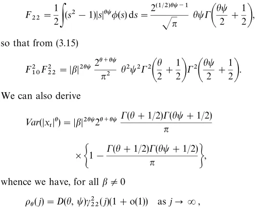
t"0.1, 0.5, 1.0, 1.5, 2.0 and 4.0. Overall, except fort"0.1,D(h, t) tends to be notably larger than C(h,b), over the range of parameter values considered, though it must be remarked thatD(h, t) is a factor ofc222 (j) notc22(j), so it by no means follows that the correspondingoh(j) will have the same ordering. The shape ofD(h,t) is very similar to that ofC(h,b), with the mode inhfalling o!
fromh"2 toh"0.5 ast, an index of nonlinearity ofx
t, increases.
Broader classes of models than (3.20) and (3.21) are, respectively,
x
t"g1tDa#bg2tDt (3.23)
and (1.4), with aO0 in each case. We stressed (3.20) and (3.21) because when
aO0 we are in Case II and deduce (3.6), which is similar to the outcome for (1.3); because unlike for (1.3) the scale factor in the approximation foroh(j) for (3.23) varies witha; and because a closed-form expression for the scale factor is only available foraO0 whenhis an even integer under (1.4), and whenhtis an even integer under (3.23).
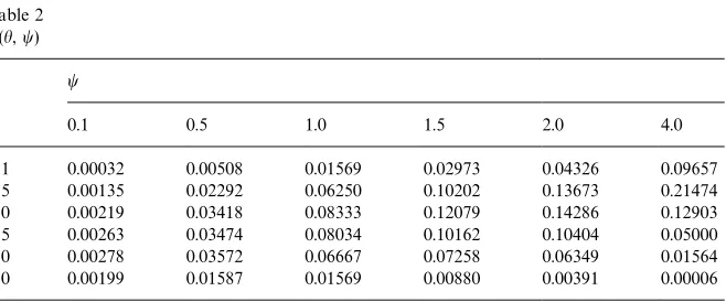
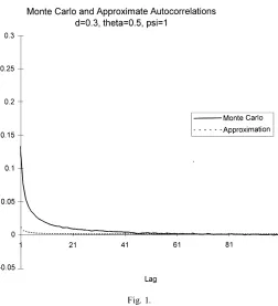
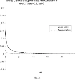
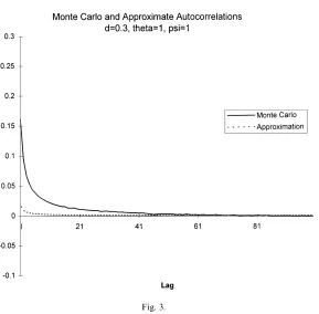
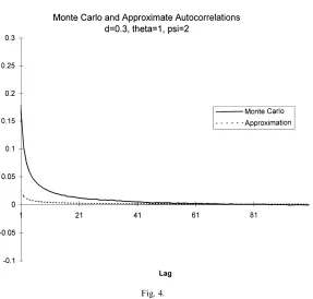
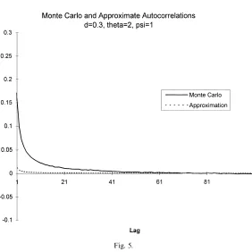
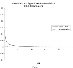
It is of interest to numerically compare our approximations with actual autocovariances. Only in very special cases are exact formulae for the latter available, so we employ Monte Carlo simulations. We considery
t"DxtDhwith
x
t given by (3.20) for b"1 and with g1t white noise and g2t the simple
fractionally integrated model (1!¸)dg2t"e
t, where¸is the lag operator,et is
white noise and 0(d(1
2(see Adenstedt, 1974). Thenc22(j) satis"es (3.9) and we
Fig. 1.
compare the approximation with the actual autocorrelations, which are cal-culated by simulation. For given d, the series g2t,t"1,2,n"1000, was
generated by the algorithm of Davies and Harte (1987). Then they
t,t"1,2,n,
were calculated for given t, h, and their sample autocorrelations at lags
j"1,2,m"100 were computed. For the givend, t, h, this process was
re-peated r"5000 times, and compared with the leading term in (3.22). We employed each combination of d"0.15, 0.3, 0.45, t"1, 2 and h"0.5, 1, 2, that is 18 cases in all, but only plot, in Figs. 1}6, the cases in whichd"0.3. The approximations, across allt, h, appear poor for lags less than 20, but later seem satisfactory, and very good for lags greater than 45. There is little sensitivity to either the nonlinearity parametert, or the transformation parameterh.
4. Further applications
Fig. 2.
4.1. Cyclic behaviour
Formulae such as (3.16) suggest that &linear' terms, when present, might sometimes be dominated by&quadratic'or higher-order terms, depending on the autocorrelation of the various latent variates. Even when this is not the case it is important to stress that"rst-order approximations may only be useful for very largej, and for more moderatejcan be improved by including terms of smaller order. The qualitative impact of such terms is notable in series with a cyclic component. Andersen and Bollerslev (1997) have found evidence of strong intraday periodicity in return volatility in foreign exchange and equity model markets. To model this kind of phenomenon, note that a lag-jautocovariance proportional to r(j; u,d)"cos(ju)j2d~1as jPR, for 0(d(1
2, 0(u(n,
has the long memory property of non-summability, but also oscillates, changing sign everyn/ulags; a class of parametric models with this property was studied by Gray et al. (1989). Supposey
tis given by (1.2) withg2t having two elements,
g(1)2t with autocorrelation decaying liker(j; 0, d
1)"j2d1~1, andg(2)2t with
auto-correlation decaying liker(j; u,d
2), for 0(u(n. Then if, for example,g1t is
Fig. 3. c(j)"Cov(y
t,yt) has linear terms in j2d1~1 and cos (ju)j2d2~1, as jPR. If
d
1'd2 then the second is of smaller order, but nevertheless its exclusion is
liable to give a misleading picture ofc(j). However, nonlinear modelling of cyclic phenomena by (1.2) needs more careful thought. For example, if two elements of
gthave lag-jautocovariance decaying liker(j;u1,d
1),r(j; u2, d2), respectively,
the theorem implies in general a contribution toc(j) decaying like
2
<
l
/1
r(j; u1, d 1)"
1
2 [cosMj(u1#u2)N#cosMj(u1!u2)N]j2d1`2d1~2. (4.1) Whend
1#d2'1/2, a second-order approximation displays cycles at
frequen-ciesu1#u
2 andu1!u2, along with linear terms with cycles atu1andu2
(when (4.1) corresponds to &squared' terms, so foru1"u
2, d1"d2, there is
Fig. 4.
4.2. Cross-sectional aggregation
For series that result from cross-sectional aggregation, such as stock indices, one might prefer to model the underlying micro-series. Suppose there aremof theseMx
itN, i"1,2,m, and the data available are
x
t" m
+
i/1 x
it, t"1, 2,2 .
Taking x
it"fi(g(ti)), where gt(i) is a p(i)]1 vector, it follows that yt"g(xt) is
of form (1.1) withg
t"(g(ti){,2,gt(m){)@if the stationaryg(ti)are spherical normal
and mutually independent. In this set-up the unitsx
it are independent across
i, but can be heterogeneous owing to possible variability with i of f
i and
C(i)(j)"Cov(g(i)
t , g(t`ji) ). We approximate c(j)"Cov(yt,yt`j) by applying the
theorem withRa block-diagonal matrix withith diagonal blockC(i)(j). In the event of some long memory in theg(ti), linear terms in theC(i)(j) will generally dominate. Units with the strongest autocorrelation will determine asymptotic behaviour, but these may give a misleading impression ofc(j) at moderatej, as they need not be the largest or most numerous. Notice that, unlessy
Fig. 5.
integerh, y
t cannot be represented as a sum of terms of the form (1.2), even if
individualx
ithave such product form, except for example if one of the functions
ofx
it is constant acrossi.
4.3. Temporal aggregation and skip-sampling
Data can be time-aggregated or skip-sampled, especially in view of the processing problems posed by the extremely long,"nely-sampled"nancial series nowadays available. The e!ect of temporal aggregation on model (1.3) in case of long memory has been considered by Andersen and Bollerslev (1997) and Bollerslev and Wright (2000). More generally, consider series z
t, t"1, 2,2 .
De"ne, form*1, the temporally aggregated series
x
t" m~1
+
s/1 z
t`s~1, t"1, 2,2.
Suppose thatz
t"g(ft) for ans]1 stationary Gaussian vector processft, such
thatEft"0,Eftf@t"I
s(so thatfthas the same basic form asgtin (1.1)). Denote
the rank of the covariance matrixXof f(m)
Fig. 6.
an r]1 vector r"Af(m)
t , where A is an r]ms matrix such that AXA@"Ir.
When s'1 it is possible that r(ms; for example, take s"2, ft"
(1!o2)~1@2(mt!om
t~1, (1!o2)1@2mt~1)@for a scalar Gaussian processmt with
zero mean, unit variance and lag-one autocorrelationo, so that we can write
z
t"g(ft)"gH(mt, mt~1) for somegHand think of the two latent variates
generat-ingz
t as consecutive variates from the same process. Now denote byyt"h(xt)
the instantaneous function of interest of the aggregated seriesx
t. Thus we have
y
t"h(g(ft)#2#g(ft`m~1))"f(gt)
for some functionf, so that we are back to precisely the situation of (1.1). On applying the Theorem, c(j)"Cov(y
t,yt`j) can be expanded in terms of the
autocovariance matrix off
t at lagsj#1!m,2, jasjPR(withm"xed), but
the rate of decay will be una!ected by the aggregation. The case of skip-sampling of a process y
t"f(gt), temporally aggregated or not, is trivially
handled. If gt is observed at intervals n'1, we deduce from the Theorem approximations for thec(nj)"Cov(y
t,yt`nj), asnjPR; this can be interpreted
for "xed jwith the sampling becoming coarser (nPR), but nis regarded as
"xed in casen"mwithmas above, where we replace each consecutive block of
m z
4.4. Jointly dependent series
It is routine to extend (1.1) to the rjointly dependent processesy
it"fi(gt),
1)i)r. Approximations for cross autocovariances between y
it and
y
k,t`j, 1)i, k)r, are then readily deduced from the Theorem. It is of interest,
however, to view this general setup in the context of a model for underlying observablesx
it,i"1)i)s. Ifxit"gi(gt), 1)i)s, andyit"gi(x1t,2,xst) is
an instantaneous function of thesex
it, then indeed we can writeyit"fi(gt). We
may wish to consider some particular structure for thex
it, such as
x
it" p1
+
k/1
g(1k)
thik(g2t), i"1,2,s,
whereg(1kt)is thekth element ofg1t, to cover multivariate extensions of (1.3) and (1.4). Notice that in order to allow for general contemporaneous correlation in
x
it,g(1kt)for anykwill in general be common to two or morexit, so that processes
y
it"DxitDh will not have the product structure (1.2). However in one case of
empirical interest (see Granger and Ding, 1996) there is a single underlying observable, s"1, but two or more functions y
it, for example y1t"xt and
y
2t"DxtDh, when product structure inxt implies the same for theyit.
5. Final comments
As much of our discussion indicates, cases when we can derive analytic formulae for scale factors of terms in our expansions are the exception rather than the rule. In simple models such as (1.4), or (3.23) withaO0 andy
t"DxtDh,
processes by applying the techniques of Hannan (1970, pp. 82}88) to the leading terms of our autocovariance expansion.
Acknowledgements
Research supported by a Leverhulme Trust Personal Research Professorship and ESRC Grant R000235892. I am grateful to Javier Hualde and Yoshihiko Nishiyama for carrying out the bulk of the numerical work reported and for the comments of referees which have led to a number of improvements.
References
Adenstedt, R., 1974. On large-sample estimation for the mean of a stationary random sequence. Annals of Statistics 2, 1095}1107.
Andersen, T.G., Bollerslev, T., 1997. Heterogeneous information arrivals of return volatility dynam-ics: increasing the long run in high frequency returns. Journal of Finance 52, 975}1006. Bollerslev, T., 1986. Generalized autoregressive conditional heteroscedasticity. Journal of
Econo-metrics 31, 302}327.
Bollerslev, T., 1987. A conditional heteroskedastic time series model for speculative prices and rates of return. Review of Economics and Statistics 69, 542}547.
Bollerslev, T., Wright, J., 2000. Semiparametric estimation of long-memory volatility dependencies: the role of high frequency data. Journal of Econometrics 98, 81}106.
Breidt, F.J., Crato, N., de Lima, P., 1998. On the detection and estimation of long memory in stochastic volatility. Journal of Econometrics 73, 325}334.
Davies, R.B., Harte, D.S., 1987. Tests for Hurst e!ect. Biometrika 74, 95}101.
Ding, Z., Granger, C.W.J., 1996. Modelling volatility persistence of speculative returns: a new approach. Journal of Econometrics 73, 185}215.
Ding, Z., Granger, C.W.J., Engle, R.F., 1993. A long memory property of stock market returns and a new model. Journal of Empirical Finance 1, 83}106.
Engle, R.F., 1982. Autoregressive conditional heteroscedasticity with estimates of the variance of United Kingdom in#ation. Econometrica 50, 987}1007.
Geweke, J., Porter-Hudak, S., 1985. The estimation and application of long memory time series models. Journal of Time Series Analysis 4, 221}238.
Granger, C.W.J., Ding, Z., 1995. Some properties of absolute returns, an alternative measure of risk. Annales d'Economie et de Statistique 40, 67}91.
Granger, C.W.J., Ding, Z., 1996. Varieties of long memory models. Journal of Econometrics 73, 61}77.
Gray, H.L., Zhang, N.F., Woodward, W.A., 1989. On generalized fractional processes. Journal of Time Series Analysis 10, 15}29.
Hannan, E.J., 1970. Multiple Time Series. Wiley, New York.
Hannan, E.J., Boston, R.C., 1972. The estimation of a nonlinear system. In: Andersson, R.S., Jennings, L.S., Ryan, D.M. (Eds.), Optimization. University of Queensland Press, St. Lucia, pp. 69}85.
Harvey, A.C., 1998. Long memory in stochastic volatility. In: Knight, J., Satchell, S. (Eds.), Forecasting volatility in"nancial markets. Butterworth-Heinemann, London.
Ibragimov, I.A., Linnik, Yu.V., 1971. Independent and Stationary Sequences of Random Variables. Wolters-Noordho!, Groningen.
Kendall, M.G., 1941. Proof of relations connected with tetrachoric series and its generalization. Biometrika 32, 196}198.
Kuznetsov, P.I., Stratonovich, R.L., Tikhonov, V.I., 1965. Nonlinear Transformations of Stochastic Processes.. Pergamon Press, New York.
Robinson, P.M., 1991. Testing for strong serial correlation and dynamic conditional heteroskedas-ticity in multiple regression. Journal of Econometrics 47, 67}84.
Robinson, P.M., 1994. Time series with strong dependence. In: Sims, C.A. (Ed.), Advances in Econometrics, Vol. 1. Cambridge University Press, Cambridge, pp. 47}95.
Robinson, P.M., 1995. Log-periodogram regression of time series with long range dependence. Annals of Statistics 23, 1048}1072.
Robinson, P.M., Za!aroni, P., 1997. Modelling nonlinearity and long memory in time series. Fields Institute Communications 11, 161}170.
Robinson, P.M., Za!aroni, P., 1998. Nonlinear time series with long memory: a model for stochastic volatility. Journal of Statistical Planning and Inference 68, 359}371.
Rosenblatt, M., 1961. Independence and dependence. In: Proceedings of the Fourth Berkeley Symposium on Mathematical Statistical and Probability. University of California Press, Ber-keley, pp. 411}443.
Sanchez de Naranjo, M.V., 1993. Non-central limit theorems for non-linear functionals ofk Gaus-sian"elds. Journal of Multivariate Analysis 44, 227}258.
Taqqu, M., 1975. Weak convergence to fractional Brownian motion and to the Rosenblatt process. Zeitschrift fu?r Wahrscheinlichkeitstheorie 31, 287}302.
Taylor, S.J., 1986. Modelling Financial Time Series. Chichester, UK.
Teyssiere, G., 1998. Nonlinear and semiparametric long-memory ARCH. Preprint.
Whistler, D.E.N., 1990. Semiparametric models of daily and intra-daily exchange rate volatility. Ph.D. Thesis, University of London.