RESEARCH ON THE THREE ANGULAR RESOLUTION
OF TERRESTRIAL LASER SCANNING
Ronghua Yang a,b,*, Xianghong Huab, Junning Liub, Hao Wuc
a
School of Civil Engineering, Chongqing University, No.174, Shazheng Street, Chongqing City, P.R.China -
[email protected]
b
School of Geodesy & Geomatics, Wuhan University, No.129, Luoyu Road, Wuhan City, Hubei Prov, P.R.China -
[email protected], [email protected]
c
School of Resources and Environmental Engineering, Wuhan University of Technology, No.129, Luoshi Road,
Wuhan City, Hubei Prov, P.R.China - [email protected]
Commission III, WG III/2
KEY WORDS: Terrestrial Laser Scanning, Angular Resolution, AMTF Model, EIFOV Model, Beamwidth, Sampling Interval
ABSTRACT:
Terrestrial laser scanning technology has been applied more and more widely in the field of Surveying and mapping. Although requirements of the accuracy for different laser scanner survey may differ considerably, spatial resolution is an important aspect, which can be divided into range and angular components. The latter is a focus of this paper and is governed primarily by scanning interval, laser beam width and angle quantisation. An ultimate goal of this research is to derive the relationship and simplified formula between scanning interval and the angular quantisation when the EIFOV(Effective Instantaneous Field of View) is equal to the scanning interval; the relationship and simplified formula of scanning interval and the angular quantisation when the EIFOV is equal to the laser beam width, and the relationship and simplified formula of the theoretical minimum EIFOV and the angular quantisation. Firstly, this paper introduces the EIFOV model and the AMTF(Average Modulation Transfer Function) model. Secondly, the dimensionless AMTF and EIFOV generic model are proposed. Thirdly, the above relathionships are deduced,which
are ellipse or hyperbola, and the three simplified formulas are proposed. The simplified formulas have direct significance on the angular resolution’s calculation and the scanning interval setting.
* Yang Ronghua, Ph.D, majors in the theory and application of terrestrial laser scanning technology, [email protected]. Project source: National Natural Science Foundation of China(NO.41174010 and No.40901214)
The Ministry of Land and Resources Sponsorship (NO.1212010914015)
This paper is a further research with some addition of more introduction of theories, on the base of my Ph.D dissertation Research on Point Cloud Angular Resolution And Processing Model of Terrestrial Laser Scanning and an early paper in Chinese Research on the point cloud angular resolution of terrestrial laser scanners, which was accepted by Geomatics and Information Science of Wuhan University and is in publication plan.
1. INTRODUCTION
The emergence of the terrestrial laser scanning technology has broken the traditional mode of surveying data acquisition and processing, and has promoted the development of the objective surface characteristics’recovery techinque which is based on the measurement model of point cloud(Reshetyuk, 2009; Zhang Yi, 2008). Recovery degree of the objective surface minuitiae feature is described generally by the spatial resolution. In terms of terrestrial laser scanning technology, the spatial resolution designates the range and angular resolution of point cloud. The latter is the main factor to determine the objective details’ recognition capability of point cloud (Lichti, 2006; Zhu Ling, 2008), which is governed primarily by scanning interval, laser beam width and angle quantisation. At present, Professor Lichi’s EIFOV(Effective Instantaneous Field of View)model, which was deduced from AMTF(Average Modulation Transfer Function) model, is the only one involving above three aspects. In practical, the angle quantisation can be changed only by selecting different scanner.. Scanning interval and laser beamwidth are usually required to determine in advance through the formula of beam width, the relationship of the
EIFOV and the scanning interval, and the EIFOV of the point cloud can be obtained. But no manufacturer of scanner provide the formula of the beam width and the range, meanwhile the relationship model among the EIFOV, scanning interval, and the angular quantisation is very complicated, so that we need to develop a simple method to calcuate the magnitude of scanning interval on the angular quantisation knowned. Furthermore, the magnitude of theoretical minimum angular resolution can be used to evaluate the instrument performance. However the theoretical minimum angular resolution is unavailable.
In order to resolve the above problems,Related research would be focused on the formulas of differenct scanner in detail: 1) The relationship and simplified formula of scanning interval and the angular quantisation when the EIFOV is equal to the scanning interval;
2) The relationship and simplified formula of scanning interval and the angular quantisation when the EIFOV is equal to the laser beam width;
3) The relationship and simplified formula of the theoretical minimum EIFOV and the angular quantisation.
The following organization of this paper is listed here:
In section 2, the basic theory is introduced including the AMTF and the EIFOV model, the three kind formulas to calculate laser beamwidth of various scanners, as well as the dimensionless AMTF and EIFOV general model.
In section 3, based on the above theory, the three angular resolution of terretrial laser scanner is researched, and it is concluded that the relationships and simplified formulas of scanning interval and the angular quantisation in two different EIFOV value, as well as the theoretical minimum EIFOV and the angular quantisation.
In section 4, the laser beamwidth and angular resolution of 29 kinds of commerical TLS systems is analysed based on the above theory.
Finally, a conclusion is drew in section 5.
2. THE METHOD OF CALCULATING BEAMWIDTH AND THE MODEL OF AMTF AND EIFOV 2.1 AMTF Model
AMTF model is computed by Fourier transfer—APSF(Average
Point Spread Function), including the sampling AMTFs, the
beam width AMTFb and quantisation AMTFq. The combined
model is(Lichti, 2006; Yang Ronghua, 2011)
1
where
Δ
= scanning interval, which unit is millimeterw
= diameter of beamwidth in the distance of S, which unit is millimeterτ
= angular quantisation, which unit is millimeteru
= frequency, which unit is 1/mm.2.2 EIFOV Model
EIFOV model is favoured for the analysis of electric-optical system resolution. The appropriate expression of the EIFOV extends to laser scanners as it quantifies the combined effects of sampling, beam width and quantisation. EIFOV model is computed via the cut-off frequency. It is(Lichti, 2006; Yang Ronghua, 2011)
where
u
c = the cut-off frequency which satisfy the equation2
2.3 Three Method of Calculating Beamwidth
The point cloud angular resolution is related with the laser beamwidth that is affected by several factors such as the scaning distance, the divergence characterization of laser beam, the diameter of the transmitting aperture and the inclination angles of the objective surface, etc(Zhang Yi, 2008;Lai Zhikai, 2004). However, no scanner manufacturer currently provides the formula used to calculate the laser beam width. Most manufacturers keep the value of the most laser characteristics parameters still as secret. So it is difficult to know how big is the beamwidth in any distance. In here three methods are given to calculate different scanner’s beam width:
Firstly, the diameter of the transmitting aperture and three more diameters in different distances are given. The formula is(Reshetyuk, 2009; Zhang Yi, 2008)
2 2 2
0
+ (
0)
w
=
w
c S
−
R
(3)where
R
0 = the range between the beam waist and thetransmitting aperture, which unit is meter
0
w
= diameter of beamwidth in the distance ofR
0, which unit is millimeterc
= constant variable, which unit is mm/mSecondly, the diameter of the transmitting aperture and the beam divergence angle is given, or two diameters in different distances are given. The formula is(Reshetyuk, 2009; Zhang Yi, 2008)
D
= diameter of the transmitting aperture, whichunit is millimeter
Thirdly, the diameter of the transmitting aperture and the diameter of beamwidth in a certain distance are given. The formula is(Reshetyuk, 2009; Zhang Yi, 2008)
2 2 2
2.4 The Dimensionless AMTF And EIFOV Generic Model
To make the model more practical and more simple, the AMTF model eq.1 and the EIFOV model eq.2 can be transformed to
dimensionless form by using variable substitution, which
satisfies the equation Δ =kw, τ=mw, u U w
= , EIFOV=Nw.
The dimensionless AMTF and EIFOV generic model is(Yang Ronghua, 2011)
where
k
= the dimensionless scanning interval, which is the ratio of the scanning interval and the beamwidthm
= the dimensionless angular quantisation, which is the ratio of the angular quantisation and the beamwidthU
= the dimensionless frequency, which is theproduct of frequency and beamwidth
c
U
= the dimensionless cut-off frequency, which is the product of cut-off frequency and beamwidthN
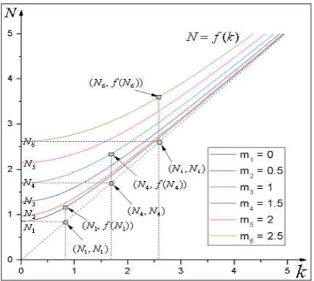
= the dimensionless EIFOV, which is the ratio of the EIFOV and the beamwidthFrom the eq.6 and eq.7, the relationship graph of the dimensionless EIFOV N and the dimensionless scanning interval k (Fig.1) can be derived, which indicates the six
relationship curve grahps of N and k under different
dimensionless angular quantisations(assumingm1=0, m2=0.5,
3 1
m = , m4=1.5, m5=2, m6=2.5). From Fig.1, we can see that N is minimum on the condition of k=0 , which is described as theoretical minimum EIFOV. Furthermore, we can also see that the function of N= f k( ) is montone increasing function, which asymptotic line is the line of N=k.
Figure 1. The rationship curve graph of N and k
3. THREE KINDS RELATIONSHIP AND SIMPLIFIED FORMULA
In practice, the scanned point cloud is supposed to have the specific angular resolution which equals scanning interval or laser beamwidth. In addition, it is hoped to evaluate the scanner performance by its theoretical minimum EIFOV which is governed only by angle quantisation. From Fig.1, the condition of the N=k is k1(or k→ +∞) can be shown, and the dimensionless EIFOV N is equal to the theoretical minimum value when k=0. Although Lichti(2006) have given that the condition of the N=1 is k=0.545, and Nmin=0.8594on the condition of ignoring angular quantisation, which can be effected when the size of angular quantisation is appropriate as scanning interval. However, more biases could arise in computing results and dimensionless variable k could not be infinite in actual scanning parameter setting, the minimum k value should be deduced(k1). Here, we assume that k1 and
2
k are the dimensionless scanning interval variables, the dimensionless EIFOV N is equal to N1 when k=k1 , the
dimensionless EIFOV N is equal to 1 when k=k2 , the
theoretical minimum dimensionless EIFOV is denoted by Nmin,
and N1 satisfy the equation
Assuming the regulations of relative approximate error is 0.005,
which is that the condition of N=k is N k 0.005
k− < . As the
relationship of N and m is montone increasing function, which asymptote is N=k and satisfy that N>k and
montone increasing function, and N k 0.005
k− < when k>k1, which is equivalent to N=k when k>k1. So we can obtain
point cloud which angular resolution is closed to scanning interval by setting the scanning interval parameter more than
1
k ,and can obtain point cloud which angular resolution is
equal to laser beamwidth by setting the scanning interval parameter at k2. Furthermore, Nmin can be used to estimate relationships of minimum theoretical angular resolution from different scanners,and use the scanner having smaller
min
N to
accomplish the task of obtaining higher angular resolution point cloud.
Analysed from above,it have great significance in deriving the
relationship of k1 and m , the relationship of k2 and m , and
the relationship of Nmin and m . Moreover, we need to derive
the simplified formula of calculating k1, k2 and Nmin under knowing the value of the angular quantisation. The following is the three kinds of relationships and simplified formulas.
3.1 The Relationship & Simplified Formula of k1 And m
With the equation (10), we can gain
With the equation (11) and (12), we can gain
1
1.9702
A
π
>
(13)With keeping two digit of decimals, indicated from the monotonicity of N and m ,derived from above deduction, the
condition which makes 1 1
1
The above equation is very complicated. we need to get its simplified form for convenient calculation. Here, the least squares curve fitting method of 1000 uniform sampling points
1
( , )m k obtained by the equation (14) is used to derive the
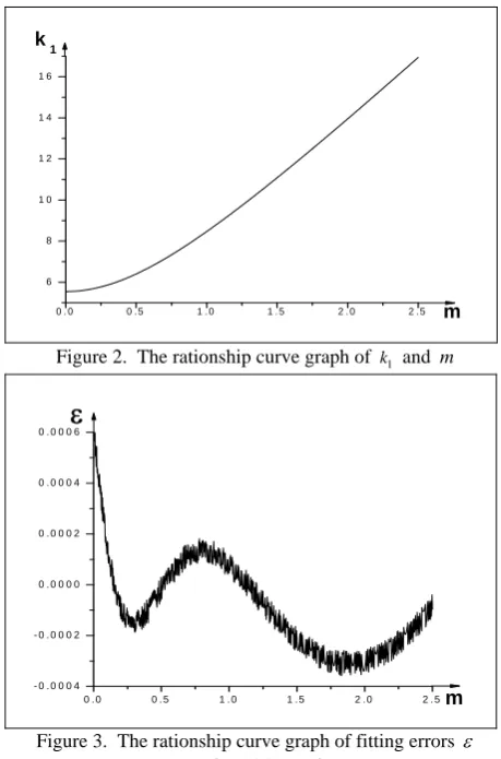
simplified formulas of k1 and m . As up to now, the highest precision in point cloud data processing of terrestrial laser scanning is 0.01 folds laser beamwidth(Zhang Yi, 2008), and the maximum angular quantisation of different scanner is 2.08 folds laser beamwidth(GIM, 2010). Therefore, we define that
[0, 2.5]
m∈ and fitting precision is 0.005. Then, we can get the relationship graph of k1 and m (Fig.2) and the fitting formulas
of k1 is
From the equation (15), we can see that the relationship graph
of k1 and m is hyperbola, and the fitting errors of the equation
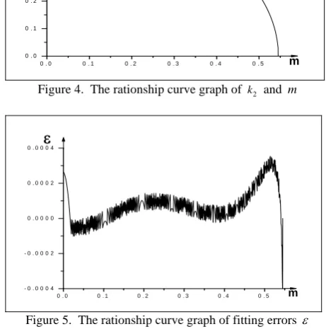
(15) and m is Fig.3. From the plot of Fig.2, we can see that fitting errors is less than 0.005 when m>0.01. so we can think that the equation (14) is approximately equaivalent with the equation (15).
Figure 3. The rationship curve graph of fitting errors ε (equation (15)) and m
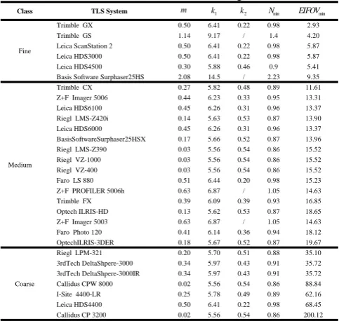
The above equation is still very complicated. Its simplified form can be derived through the same method as above. we can get the relationship graph of k2 and m ( Fig.4) and the fitting
From the equation (17), the relationship graph of k1 and m is ellipse, and the fitting errors of the equation (17) and m is Fig.5. From the plot of Fig.5, we can see that fitting errors is less than 0.0003. so we can think that the equation (16) is approximately equaivalent with the equation (17).
0 . 0 0 . 1 0 . 2 0 . 3 0 . 4 0 . 5 0 . 0
0 . 1 0 . 2 0 . 3 0 . 4 0 . 5 k2
m
Figure 4. The rationship curve graph of k2 and m
0 . 0 0 . 1 0 . 2 0 . 3 0 . 4 0 . 5 - 0 . 0 0 0 4
- 0 . 0 0 0 2 0 . 0 0 0 0 0 . 0 0 0 2 0 . 0 0 0 4
ε
m
Figure 5. The rationship curve graph of fitting errors ε (equation (17)) and m
3.3 The Relationship & Simplified Formula ofNminAndm
With the equation (6), (7) and k=0 , we can gain the
relationship of Nmin and m that is
1
min min
min min
2 (
) sin(
)
2
2
2
2
2
m
J
N
N
m
N
N
π
π
π
π
=
π
(18)The equation (18) is needed to simplify using the same method as above. we can also get the relationship graph of Nmin and
m ( Fig.6) and the fitting formulas of Nmin and m that is
N
min=
a
3+ ⋅ −
b
3(
m
g
3)
2−
h
3 (19) wherea
3 = 0.821023
b
= 1.038143
g
= 0.03713
h
= 0.0437From the equation (19), the relationship graph of k1 and m is hyperbola, and the fitting errors of the equation (19) and m is Fig.7. From the plot of Fig.7, we can see that fitting errors is
less than 0.004. So the equation (18) is approximately equaivalent with the equation (19).
0 . 0 0 . 5 1 . 0 1 . 5 2 . 0 2 . 5 0 . 0
0 . 5 1 . 0 1 . 5 2 . 0 2 . 5
( 0 , 0 . 8 5 9 4 )
Nm i n
m
Figure 6. The rationship curve graph of Nmin and m
0 . 0 0 . 5 1 . 0 1 . 5 2 . 0 2 . 5 - 0 . 0 0 2
- 0 . 0 0 1 0 . 0 0 0 0 . 0 0 1 0 . 0 0 2 0 . 0 0 3 0 . 0 0 4
ε
m
Figure 7. The rationship curve graph of fitting errors ε (equation (19)) and m
4. BEAMWIDTH AND RESOLUTION OF TLS SYSTEM
The laser beam width and angular resolution of 29 commerically available TLS systems(GIM, 2010) is analysed using the three methods of calculating beamwidth diameter and the equation (15), (17), (19). To facilitate the comparision, each vendor’s reported finest angular sampling interval and beamwith and calculated EIFOV have been reduced to linear spatial units at a range of 50m. The results about the coefficients of different scanner’s beamwidth formula are given in Table 1, and the results about k1, k2 and Nmin of different scanner are given in Table 2.
From Table 1, we can see that the three methods of equation (3), (4) and (5) can solve the problem of calculating all TLS systems’ laser beamwidth diameter.
Shown as Tab. 2:
1) The 29 systems can be classified into three groups
according to EIFOVmin (the theoretical minimum EIFOV): fine resolution scanners; medium resolution instruments; and coarse resolution instruments.
2) For Trimble GS、Basis Software Surphaser 25HS、Z+F
PROFILER 5006h 和 Z+F Imager 5003: The theoretical
minimum dimensionless EIFOV N(>1); The dimensionless angular quantisation(≤0.545); The dimensionless scanning interval k2(N/A);
3) For other scanners: The theoretical minimum dimensionless EIFOV N(<1); The dimensionless angular quantisation(≤0.545);
4) For Riegl LMS-Z390, Riegl VZ-1000, Riegl VZ-400,
Callidus CPW8000, Callidus CP320: Nmin and k1 achieve
minimum values, k1=5.56, Nmin=0.86;
5) For Basis Software Surphase:
min
N and k1 achieve maximum values, k1=14.43, Nmin=2.23;
6) For Faro LS880: k2 achieve minimum values, k2=0.2; 7) The size of spot diameter affects a lot on minimum angular
resolution, which arises the most in low-precision scanners. Furthermore, angular resolution of point cloud is as an integrated result of scanning interval, angular accuracy and spot diameter. Meanwhile, the method of spot-overlay can improver angular resolution of point cloud, with a maximum value of 0.86 times of spot diameter.
Table 1. The coefficient of the formulas of different scanner’s
beamwidth diameter
Method TLS System D0 γ R0 w0 c
Firtst
Basis Software Surphaser 25HS 2.8 4.52 2.32 0.3481 BasisSoftware Surphaser 25HSX 2.8 4.52 2.32 0.3481 Leica ScanStation 2 6 25 4.00 0.1789
the dimensionless theoretical minimum angular resolution
Class TLS System m k1 k2 Nmin EIFOVmin BasisSoftwareSurphaser25HSX 0.17 5.66 0.52 0.87 13.96 Riegl LMS-Z390 0.03 5.56 0.54 0.86 15.52 OptechILRIS-3DER 0.18 5.67 0.52 0.87 19.67
Coarse
Riegl LPM-321 0.20 5.70 0.51 0.88 35.10 3rdTech DeltaShpere-3000 0.34 5.97 0.43 0.91 35.72 3rdTech DeltaShpere-3000IR 0.34 5.97 0.43 0.91 35.72 Callidus CPW 8000 0.02 5.56 0.54 0.86 88.84 I-Site 4400-LR 0.25 5.78 0.49 0.89 62.16 Leica HDS4400 0.50 6.41 0.22 0.98 68.45 Callidus CP 3200 0.02 5.56 0.54 0.86 200.12
5. CONCLUSIONS
Spatial resolution governs the level of identifiable detail within a scanned point cloud and is particularly important for recording of objective features with fine details(Lichti,2006). The angular resolution of laser scanners is affected by sampling interval, laser beamwidth and angular quantisation. EIFOV is regarded as a more appropriate measure of the angualr resolution. To quickly obtain scanning interval corresponding with the known angular resolution, here we present the dimensionless AMTF and EIFOV generic model, the three kind methods of calculating beamwidth diameter, and the three kind functional relationship that is the relationship of k1 and
m where N=k, the relationship of k2 and m where N=1,
and the relationship of Nmin and m where k=0. In addition, we derive the above relationsips’ simplified formula, give the definition of the optimal sampling interval, and analyse 29 available TLS systems’ laser beamwidth diameter and variablesk1 , k2and Nmin. The results shows that the simplified formulas have direct significance on the angular resolution’s calculation and the scanning interval setting.
ACKNOWLEDGMENT
The authors would like to thank Prof. Xianghong Hua of Wuhan University for his professional expertis and efforts in supporting this research work. The other acknowlegment goes to Associate professor Xing Liu of Chongqing University and Dr. Junning Liu of Wuhan University for their help.
REFERENCES
Mathias Lemmens, 2010. The fourth Product Survey on Terrestrial Laser Scanners “Terrestrial Laser Scanners, August
2010”, GIM International.
http://www.gim-international.com/productsurvey/id41-Terrestrial_Laser_Scanners,_August.html (August. 2010).
Lai Zhikai, 2004. Accuracy analysis and calibration of ground-based laser scanners. Master thesis in Geodesy, National Chenggong University, pp.11-21.
Lichti D.D, 2006. Angular resolution of terrestrial laser scanners. Photogrammetric, 21(14), pp. 141-160.
Reshetyuk Y, 2009. Self-calibration and direct georeferencing in terrestrial laser scanning. Doctoral thesis in Geodesy, Royal Institute of Technology, pp. 10-15.
Yang Ronghua, Hua Xianghong, Qiu Weiing, Tang Kun and Geng Tao, 2011. Research on the terrestrial laser scanners’s angular resolution of any direction. Journal of Geomatics, 36(3) , pp. 11-12,54.
Zhang Yi, 2008. Research on Point Cloud Processing of Terrestrial Laser Scanning. Doctoral thesis in Geodesy, Wuhan University, pp. 1-16, 24-28.
Zhu Ling and Shi Ruoming, 2008. Research on the point cloud resolutioins of TLS. Journal of Remote Sensing, 12(3) , pp. 405-410.