de Bordeaux 18(2006), 537–557
Bases of canonical number systems in quartic
algebraic number fields
parHorst BRUNOTTE, Andrea HUSZTI etAttila PETH ˝O
Dedicated to Professor Michael Pohst on the occasion of his60th birthday
R´esum´e. Les syst`emes canoniques de num´eration peuvent ˆetre consid´er´es comme des g´en´eralisations naturelles de la num´eration classique des entiers. Dans la pr´esente note, une modification d’un algorithme de B. Kov´acset A. Peth˝oest ´etablie et appliqu´ee au calcul des syst`emes canoniques de num´eration dans certains anneaux d’entiers de corps de nombres alg´ebriques. L’algorithme permet de d´eterminer tous les syst`emes canoniques de num´eration de quelques corps de nombres de degr´e quatre.
Abstract. Canonical number systems can be viewed as natu-ral genenatu-ralizations of radix representations of ordinary integers to algebraic integers. A slightly modified version of an algorithm of B. Kov´acsand A. Peth˝ois presented here for the determina-tion of canonical number systems in orders of algebraic number fields. Using this algorithm canonical number systems of some quartic fields are computed.
1. Introduction
The investigation of the question wether an algebraic number field is monogenic is a classical problem in algebraic number theory (cf. [9]). Ac-cording to B. Kov´acs [19] the existence of a power integral basis in an algebraic number field is equivalent to the existence of a canonical number system for its maximal order. Moreover, using a deep result ofK. Gy˝ory
[13] on generators of orders of algebraic number fields B. Kov´acs [19] proved that up to translation by integers there exist only finitely many canonical number systems in the maximal order of an algebraic number field.
LetR be an order of an algebraic number field andα∈R. 1
Research was supported in part by grant T67580 of the Hungarian National Foundation for Scientific Research
Manuscrit re¸cu le 10 janvier 2006.
Definition. (cf. [3], Definition 4.1, [5]) The algebraic integerαis called a basis of a canonical number system (or CNS basis) forR if every nonzero element ofR can be represented in the form
n0+n1α+· · ·+nlαl
withni∈ {0, . . . ,|N ormQ(α)|Q(α)| −1}, nl 6= 0.
Canonical number systems can be viewed as natural generalizations of radix representations of ordinary integers (V. Gr¨unwald[12]) to algebraic integers. Originating from observations ofD. E. Knuth[17] (see also [18], Ch. 4) the theory of canonical number systems was developed byI. K´atai
andJ. Szab´o[16],B. Kov´acs[19],I. K´ataiandB. Kov´acs([14], [15]),
W. J. Gilbert[10] and others. There are connections to the theories of finite automata (see e.g. K. Scheicher [30], J. M. Thuswaldner[32]) and fractal tilings (see e.g. S. Akiyama and J. M. Thuswaldner [5]). RecentlyS. Akiyama et al. [2] put canonical number systems (CNS) into a more general framework thereby opening links to other areas, e.g. to a long-standing problem on Salem numbers.
B. Kov´acs and A. Peth˝o [20] established an algorithm for finding all CNS bases of monogenic algebraic number fields (see also [27] for a com-prehensive description of this algorithm and its background). In this note we present a slightly modified version of this algorithm for the determi-nation of CNS bases of orders of algebraic number fields. The method is exploited here for some families of number fields of low degrees; our main applications are cyclotomic and simple fields of degree four. CNS bases in quadratic number fields were described by several authors (see [14],[15],[10],[11],[32],[4] and others); further, CNS bases are explicitely known for some cubic and quartic fields ([20], [3], [27]). The list of CNS bases of simplest cubic fields given in [3] is extended in the present note too.
The authors wish to express many thanks to Professors S. Akiyama and J. M. Thuswaldner for their constant support.
2. CNS bases of algebraic number fields
In the sequel we denote by Q the field of rational numbers, by Z the set of integers and by N the set of nonnegative integers. For an algebraic integerγ we letµγ ∈Z[X] be its minimal polynomial andCγ the set of all
CNS bases for Z[γ]. We denote by C the set of CNS polynomials; for the general definition of CNS polynomials we refer the reader to A. Peth˝o
[25], however, for our purposes it suffices to keep in mind that α is a CNS basis forZ[α] if and only ifµα is a CNS polynomial. It can algorithmically
B. Kov´acs [19] introduced the following set of polynomials K={pdXd+pd−1Xd−1+· · ·+p0 ∈Z[X]|
d≥1,1 =pd≤pd−1≤. . .≤p1 ≤p0 ≥2} which plays a decisive role in the theory of CNS polynomials (see [1], The-orem 2.3).
Lemma 2.1. (B. Kov´acs – A. Peth˝o)For every nonzero algebraic in-teger α the following constants can be computed effectively:
kα= min{k∈Z|µα(X+n)∈ K for alln∈Z withn≥k}, cα = min{k∈Z|µα(X+k)∈ C}.
Proof. See [20], Section 5.
Note thatcα ≤kα by ([19], Lemma 2) and that ifβ is a conjugate of α
thenkβ =kα and cβ =cα.
Corollary 2.1. If α is a CNS basis for an orderR thencα ≤0, α−cα is
a CNS basis forR, butα−cα+ 1is not a CNS basis for R.
Proof. This is clear by the definitions.
To a polynomialP(X) =pdXd+pd−1Xd−1+· · ·+p0∈Z[X], pd= 1 we
associate the mappingτP =τ :Zd→Zddefined by τP(A) =
−
p1A1+· · ·+pdAd p0
, A1, . . . , Ad−1
,
whereA= (A1, . . . , Ad)∈Zd. This turned out very useful to proveP(X)∈
C. Indeed Brunotte [7] proved the following theorem, that gives an efficient algorithm for testing if a polynomial is CNS or not.
Theorem 2.1. Assume that E ⊆Zd has the following properties:
(i) (1,0, . . . ,0)∈E,
(ii) −E ⊆E,
(iii) τ(E)⊆E,
(iv) for every e∈E there exist some l >0 withτl(e) = 0.
ThenP(X)∈ C.
The following notion seems to be convenient for the intentions of the present note.
Definition. The algebraic integerα is called a fundamental CNS basis for
R if it satisfies the following properties:
Theorem 2.2. Let γ be an algebraic integer. Then there exist finite effec-tively computable disjoint subsets F0(γ),F1(γ)⊂ Cγ with the properties:
(i) For everyα ∈ Cγ there exists somen∈Nwithα+n∈ F0(γ)∪F1(γ).
(ii) F1(γ) consists of fundamental CNS bases forZ[γ].
Proof. By ([20], Theorem 5) there exist finitely many effectively computable
α1, . . . , αt∈Z[γ], n1, . . . , nt∈Z, N1, . . . , Nt⊂Z, N1, . . . , Ntfinite
such that for everyα∈Z[γ] we have
α∈ Cγ ⇐⇒
(2.1)
α=αi−h for somei∈ {1, . . . , t}, h∈Z and h≥ni orh∈Ni.
Therefore the set
F :={αi−ni|i= 1, . . . , t} ∪ t [
i=1
{αi−h|h∈Ni}
is a finite effectively computable subset ofCγ.
For everyα∈F let
Mα ={m∈Z|m≤kα, α−k∈ Cγ for all k=m, . . . , kα}.
Observing m ≥cα for all m ∈ Mα we see using Lemma 2.1 that Mα is a
nonempty finite effectively computable set. Let
mα= minMα
and
F0(γ) ={α−cα|α∈F, mα> cα}, F1(γ) ={α−cα|α∈F, mα=cα}.
We show that F1(γ) consists of fundamental CNS bases for Z[γ]. Let
ϕ∈ F1(γ), henceϕ=α−cα with some α∈F. By Corollary 2.1 we have ϕ∈ Cγ, ϕ+ 1∈ C/ γ. Forn∈Nwe find
ϕ−n=α−(mα+n)∈ Cγ,
because for mα +n ≤ kα this is clear by the definition of mα, and for mα +n > kα we have µϕ−n = µα(X + (mα +n)) ∈ K and therefore ϕ−n∈ Cγ by ([19], Lemma 2).
Letβ ∈ Cγ. By (2.1) there are i∈ {1, . . . , t}and h∈Zwith β =αi−h and h≥ni orh∈Ni.
If h ∈ Ni then β ∈ F and β−cβ ∈ F0(γ)∪ F1(γ) by Corollary 2.1. If h≥ni then α=αi−ni ∈F, h−ni−cα ∈Nand
β+ (h−ni−cα) =α−cα∈ F0(γ)∪ F1(γ).
Remark. Note thatϕ∈ F0(γ) impliesϕ−n∈ F1(γ) for somen∈N\ {0}. Therefore the theorem ofB. Kov´acs([19], Lemma 2) can be rephrased in the following form: An algebraic number field is monogenic if and only if there exists a fundamental CNS basis for its maximal order.
Slightly modifying the algorithm ofB. Kov´acsand A. Peth˝o [20] we now present the algorithm for finding the above mentioned sets F0(γ) and F1(γ). The (finite) set T is introduced to keep track of the calculations performed; in some cases (see e.g. Theorem 3.1) the amount of computa-tions can thereby be reduced. Recall that algebraic integersα, β are called equivalent if there is somez∈Zsuch that β =z±α (see e.g. [9]).
Algorithm 2.1. (CNS basis computation)
[Input] A nonzero algebraic integer γ and a (finite) set B of represen-tatives of the equivalence classes of generators of power integral bases of
Z[γ].
[Output]The sets F0(γ) and F1(γ).
(1.) [Initialize]Set{β1, . . . , βt}=B ∪(−B),F0 =F1 =T =∅and i= 1. (2.) [Compute minimal polynomial] ComputeP =µβi.
(3.) [Element of F0 ∪F1 found?] If there exist k ∈ Z, δ ∈ {0,1} with (P, k, δ)∈T insertβi−kinto Fδ and go to step 11.
(4.) [Determine upper and lower bounds]Calculate kβi and cβi.
(5.) [Insert element into F1?] If kβi −cβi ≤ 1 insert βi−cβi into F1,
(P, cβi,1) into T and go to step 11, else perform step 6 for l = cβi +
1, . . . , kβi−1, put pkβi = 1, k=cβi and go to step 8.
(6.) [Check CNS property] If P(X+l) ∈ C set pl = 1, otherwise set pl= 0.
(7.) [Check CNS basis condition] If pk= 0 then go to step 9.
(8.) [Insert element intoF0∪F1] If pk+1 =· · ·=pkβi = 1 insertβi−k
into F1, (P, k,1) into T and go to step 11, else insert βi−k into F0 and (P, k,0)into T.
(9.) [Next value ofk]Set k←k+ 1.
(11.) [Next generator] Set i←i+ 1.
(12.) [Finish?] If i≤t then go to step 2.
(13.) [Terminate]Output F0(γ) =F0 andF1(γ) =F1 and terminate the
algorithm.
We verify that the algorithm above delivers all CNS bases of a given order Z[γ].
Theorem 2.3. Let γ be a nonzero algebraic integer and B a set of repre-sentatives of the equivalence classes of generators of power integral bases of
Z[γ]. Then Algorithm 2.1 computes the sets F0(γ),F1(γ) with properties (i) and (ii) of Theorem 2.2.
Proof. It is easy to see thatF0(γ)∪ F1(γ)⊂ Cγ and thatF1(γ) consists of
fundamental CNS bases forZ[γ]. Let α ∈ Cγ, hence α =n+β with some n ∈ Z, β ∈ B ∪(−B). Clearly, −n ≥ cβ. By construction there is some
integerk∈[cβ, kβ] with β−k∈ F0(γ)∪ F1(γ). Letl1, . . . , ls ∈[cβ, kβ] be
exactly those indices withplσ = 0 (σ = 1, . . . , s) andcβ < p1 < . . . < ps < kβ. If−n≥ls+ 1 thenϕ=β−(ls+ 1)∈ F1(γ) andα=ϕ−(−n−(ls+ 1)).
Finally, let−n < ls+ 1, and observe that−n /∈ {l1, . . . , ls}. Then −n < l1 orlσ <−n < lσ+1 for someσ ∈ {1, . . . , s−1}imply α∈ F0(γ). The following example illustrates the application of Algorithm 2.1. For polynomials outside the setK the CNS property was checked by the algo-rithm described in [7] (an improved version of this algoalgo-rithm was imple-mented byT. Borb´ely [6]).
Remark. Note that if cβ < kβ and µβ(X + k) ∈ C for all k ∈
{cβ+ 1, . . . , kβ−1} then−cβ+β ∈ F1(γ). Lemma 2.2. Let k∈Z.
(i) For fk=f(X+k) withf =X3−X+ 3∈Z[X]we have fk ∈ K ⇐⇒ k≥3
and
fk∈ C ⇐⇒ k= 0 or k≥2.
(ii) For fk=f(X+k) withf =X3−X−3∈Z[X]we have fk ∈ K ⇐⇒ k≥4
and
(iii) For fk=f(X+k) withf =X3−2X2−69X−369∈Z[X]we have fk∈ K ⇐⇒ k≥13 ⇐⇒ fk∈ C.
(iv) For fk=f(X+k) withf =X3+ 2X2−69X+ 369∈Z[X]we have fk ∈ K ⇐⇒ k≥5
and
fk∈ C ⇐⇒ k≥4.
Proof. (i) The first statement is clear because fk = X3 + 3kX2 +
(3k2 −1)X +k3 −k+ 3. Using this, Gilbert’s theorem (see [3], Theo-rem 3.1) and ([3], Proposition 3.12) the second statement follows.
(ii) The first statement is clear because fk = X3+ 3kX2+ (3k2−1)X+ k3−k−3. Using this and Gilbert’s theorem (see [3], Theorem 3.1) and checking f3∈ C the second statement follows.
(iii) Clearly, k < 13 implies fk =X3+ (3k−2)X2+ (3k2−4k−69)X+ k3−2k2−69k−369∈ K ∪ C/ .
(iv) Observingfk=X3+(3k+2)X2−(3k2+4k−69)X+k3+2k2−69k+369
and checkingf4 ∈ C these statements can be proved analogously. For a monogenic algebraic number field K we write Fδ(K) instead of
Fδ(γ) whereγ is some generator of a power integral basis ofK (δ ∈ {0,1}). Example. Letϑbe a root of the polynomialX3−X+ 3∈Z[X]. By ([9], Section 11.1) up to equivalence all generators of power integral bases of Z[ϑ] are given byϑand −5ϑ+ 3ϑ2.By Lemma 2.2 we havec
ϑ= 0, kϑ= 3,
and therefore by Algorithm 2.1
ϑ∈ F0(Q(ϑ)),−2 +ϑ∈ F1(Q(ϑ)).
Analogously, we have µ−ϑ=X3−X−3, c−ϑ= 3, k−ϑ= 4,and then
−3 +ϑ∈ F1(Q(ϑ)).
Similarly, we haveµ−5ϑ+ϑ2 =X3−2X2−69X−369, c
−5ϑ+ϑ2 =k
−5ϑ+ϑ2 = 13,and
−13−5ϑ+ϑ2∈ F1(Q(ϑ)),
and finallyµ5ϑ−ϑ2 =X3+ 2X2−69X+ 369, c5ϑ
−ϑ2 = 4, k5ϑ
−ϑ2 = 5,and −4 + 5ϑ−ϑ2∈ F1(Q(ϑ)).
Collecting our results we findF0(Q(ϑ)) ={ϑ} and
F1(Q(ϑ)) ={−2 +ϑ,−3−ϑ,−13−5ϑ+ϑ2,−4 + 5ϑ−ϑ2}.
In some cases the determination of CNS bases is considerably easier if
Proposition 2.1. Let γ be a nonzero algebraic integer with at least one real conjugate and B a set of representatives of the equivalence classes of generators of power integral bases of Z[γ].
(i) For α∈Z[γ]\ {0} we havecα≥M(α) + 2and c−α≥ −m(α) + 1.
(ii) Let β ∈ B. Then β −M(β)−2 ∈ F1(γ) if µβ−M(β)−2 ∈ K, and −β+m(β)−1∈ F1(γ) if µ−β+m(β)−1 ∈ K.
(iii) If µβ−M(β)−2, µ−β+m(β)−1 ∈ K for all β ∈ B then we haveF0(γ) =∅
and
F1(γ) =
β−M(β)−2,−β+m(β)−1|β ∈ B .
Proof. (0) For everyα∈Z[γ] we have real embeddingsτα, ρα ofQ(γ) with M(α)≤τα(α), ρα(α)< m(α) + 1.
(i) Assumecα =M(α) + 2−kfor somek∈N\ {0}. Thenµα(X+M(α) +
2−k)∈ C, thus by ([1], Theorem 2.1)
τα(α)−(M(α) + 2−k)<−1
which by (0) yields the contradiction
M(α)< M(α)−k+ 1.
The other inequality is proved analogously.
(ii) It is enough to show that (β−M(β)−2) + 1,(−β+m(β)−1) + 1∈ C/ . In view of ([1], Theorem 2.1) this is clear because by (0)
τβ(β−M(β)−1) =τβ(β)−M(β)−1≥M(β)−M(β)−1 =−1, ρβ(−β+m(β))>−m(β)−1 +m(β) =−1.
(iii) Denoting byF =
β−M(β)−2,−β+m(β)−1|β ∈ B it suffices to show that
Cγ⊂ϕ−n|ϕ∈F, n∈N .
Let α ∈ Cγ, β ∈ B, n ∈ Z with α = n±β. In case α = n+β we have
−M(β)−2−n∈Nby (0) and
α+ (−M(β)−2−n) =β−M(β)−2∈F,
and in caseα=n−β we analogously find m(β)−1−n∈Nand
α+ (m(β)−1−n) =−β+m(β)−1∈F.
3. CNS bases in quadratic and cubic number fields
We conclude our observations by computing F0 and F1 of several qua-dratic, cubic and quartic number fields. For the sake of completeness we start with the formulation of some well-known results in our language.
CNS bases of quadratic number fields were studied by several authors (see [14],[15],[10], [11], [32],[4] and others).
Theorem 3.1. (I. K´atai – B. Kov´acs, W. J. Gilbert) Let D 6= 0,1
Proof. A representative of the generators of power integral bases of Q(ϑ) is given by β = 1+ϑ follow from Proposition 2.1 and ([10], Theorem 1). For D < 0 Algorithm 2.1 and ([10], Theorem 1) yield the assertions.
Using a theorem ofS. K¨ormendi[21]S. Akiyamaet al. ([3], Theorem 4.5) described all CNS in a family of pure cubic number fields.
Theorem 3.2. (S. K˝ormendi – S. Akiyama et al.) Let m ∈ N\ {0}
be not divisible by 3 and m3+ 1 squarefree. For ϑ = √3
m3+ 1 we have F0(Q(ϑ)) =∅ and
F1(Q(ϑ)) ={−ϑ,−m−2 +ϑ,−2m2−2 +mϑ+ϑ2,−m2−2−mϑ−ϑ2}.
Theorem 3.3. (S. Akiyama et al.) Let t ∈Z, t ≥ −1 and ϑ denote a root of the polynomial
X3−tX2−(t+ 3)X−1.
Then we haveF0(Q(ϑ)) =∅ and
F1(Q(ϑ)) ={−3−ϑ,−t−5−tϑ+ϑ2,−1 + (t+ 1)ϑ−ϑ2} ∪ G ∪ G−1∪ G0∪ G2
where
G= (
{−t−3 +ϑ,−1 +tϑ−ϑ2,−t−5−(t+ 1)ϑ+ϑ2}, if t≥0, ∅ otherwise,
G−1 =
{−3 +ϑ,−2−ϑ−ϑ2,−5 +ϑ2,−19 + 9ϑ+ 4ϑ2,−5−9ϑ−4ϑ2 −22 + 5ϑ+ 9ϑ2,−2−5ϑ−9ϑ2,−25−4ϑ+ 5ϑ2,1 + 4ϑ−5ϑ2,
−7−ϑ+ϑ2,−1 +ϑ−ϑ2,−6 + 2ϑ+ϑ2,−2−2ϑ−ϑ2,
−6 +ϑ+ 2ϑ2,−2−ϑ−ϑ2}, if t=−1, ∅ otherwise,
G0 =
{−9 + 2ϑ+ϑ2,−2−2ϑ−ϑ2,−11−3ϑ+ 2ϑ2,−1 + 3ϑ−2ϑ2,
−10−ϑ+ 3ϑ2,−1 +ϑ−3ϑ2}, if t= 0,
∅ otherwise,
G2 =
{−37 + 3ϑ+ 2ϑ2,−2−3ϑ−2ϑ2,−42−20ϑ+ 9ϑ2,
3 + 20ϑ−9ϑ2,−43−23ϑ+ 7ϑ2,−4 + 23ϑ−7ϑ2}, ift= 2, ∅ otherwise.
Proof. We proceed similarly as in Example 2, but leave the verifications of computational details to the reader. By [9] up to equivalence all generators of power integral bases ofZ[ϑ] are the following:
• for arbitrary t: ϑ,−tϑ+ϑ2,(t+ 1)ϑ−ϑ2;
• fort=−1 additionally: 9ϑ+ 4ϑ2,5ϑ+ 9ϑ2,−4ϑ+ 5ϑ2,−ϑ+ϑ2,2ϑ+
ϑ2, ϑ+ 2ϑ2;
• fort= 0 additionally: 2ϑ+ϑ2,−3ϑ+ 2ϑ2,−ϑ+ 3ϑ2; • fort= 2 additionally: 3ϑ+ 2ϑ2,−20ϑ+ 9ϑ2,−23ϑ+ 7ϑ2.
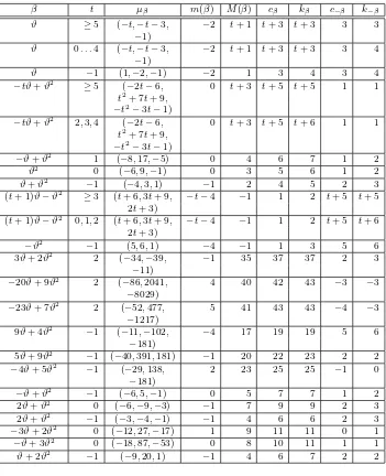
The proof is now accomplished by Proposition 2.1 and Table 1 below where we use the following notation: β is a generator of a power integral basis of Q(ϑ). The minimal polynomialµβ =X3+a1X2+a2X+a3ofβ is given by (a1, a2, a3). Lower bounds for the constantscβ, kβ are given by Proposition
2.1. For their determination ([3], Theorem 3.1) and ([8], Theorem 5.1) are used. Observe that in all cases considered here Remark 2 applies if
β t µβ m(β) M(β) cβ kβ c−β k−β
ϑ ≥5 (−t,−t−3, −2 t+ 1 t+ 3 t+ 3 3 3
−1)
ϑ 0. . .4 (−t,−t−3, −2 t+ 1 t+ 3 t+ 3 3 4
−1)
ϑ −1 (1,−2,−1) −2 1 3 4 3 4
−tϑ+ϑ2
≥5 (−2t−6, 0 t+ 3 t+ 5 t+ 5 1 1
t2
+ 7t+ 9,
−t2
−3t−1)
−tϑ+ϑ2
2,3,4 (−2t−6, 0 t+ 3 t+ 5 t+ 6 1 1 t2
+ 7t+ 9,
−t2
−3t−1)
−ϑ+ϑ2
1 (−8,17,−5) 0 4 6 7 1 2
ϑ2
0 (−6,9,−1) 0 3 5 6 1 2
ϑ+ϑ2
−1 (−4,3,1) −1 2 4 5 2 3
(t+ 1)ϑ−ϑ2
≥3 (t+ 6,3t+ 9, −t−4 −1 1 2 t+ 5 t+ 5
2t+ 3) (t+ 1)ϑ−ϑ2
0,1,2 (t+ 6,3t+ 9, −t−4 −1 1 2 t+ 5 t+ 6 2t+ 3)
−ϑ2
−1 (5,6,1) −4 −1 1 3 5 6
3ϑ+ 2ϑ2
2 (−34,−39, −1 35 37 37 2 3
−11)
−20ϑ+ 9ϑ2
2 (−86,2041, 4 40 42 43 −3 −3
−8029)
−23ϑ+ 7ϑ2
2 (−52,477, 5 41 43 43 −4 −3
−1217) 9ϑ+ 4ϑ2
−1 (−11,−102, −4 17 19 19 5 6
−181) 5ϑ+ 9ϑ2
−1 (−40,391,181) −1 20 22 23 2 2
−4ϑ+ 5ϑ2
−1 (−29,138, 2 23 25 25 −1 0
−181)
−ϑ+ϑ2
−1 (−6,5,−1) 0 5 7 7 1 2
2ϑ+ϑ2
0 (−6,−9,−3) −1 7 9 9 2 3
2ϑ+ϑ2
−1 (−3,−4,−1) −1 4 6 6 2 3
−3ϑ+ 2ϑ2
0 (−12,27,−17) 1 9 11 11 0 1
−ϑ+ 3ϑ2
0 (−18,87,−53) 0 8 10 11 1 1
ϑ+ 2ϑ2
−1 (−9,20,1) −1 4 6 7 2 2
Table 1
4. CNS bases in quartic cyclotomic fields
In this section we treat the cyclotomic fields of degree 4.
Theorem 4.1. Let ζ be a primitive eighth root of unity. Then we have
F0(Q(ζ)) =∅ and
Proof. By R. Robertson [29] up to equivalence all generators of power integral bases of Q(ζ) are given by ζk, k ∈ Z, k odd. Observing µ
ζ = X4 + 1 one immediately finds kζ = 4. The algorithm described in [7]
and ([4], Theorem 5.4) yield cζ = 3, and a straightforward application of
Algorithm 2.1 concludes the proof.
Theorem 4.2. Let ζ be a primitive twelfth root of unity. Then we have
F0(Q(ζ)) =∅ and
F1(Q(ζ)) ={−3+ζ,−3−ζ,−3+ζ−1,−3−ζ−1,−1−ζ2+ζ−1,−2+ζ2−ζ−1}.
Proof. The proof works analogously as that of Theorem 4.1. Theorem 4.3. Let ζ be a primitive fifth root of unity. Then we have
F0(Q(ζ)) =∅ and
F1(Q(ζ)) ={−2 +ζ,−3−ζ,−2 +ζ+ζ3,−3−ζ−ζ3}.
Proof. By [28] up to equivalence all generators of power integral bases of Z[ζ] areζ and 1+1ζ. One immediately checks that
fk(X) =µζ(X+k)∈ K ⇐⇒ k≥4,
hencekζ = 4. By ([4], Theorem 5.4) one findsk≥ −5 forfk∈ C. Trivially, f0, f−1 ∈ C/ , and an application of the algorithm described in [7] yields
fk∈ C/ for k=−5,−4,−3,−2,1, butf2, f3∈ C. Thus we have shown that
fk∈ C ⇐⇒ k≥2,
hencecζ = 2 and fk∈ C for all k∈ {cζ, . . . , kζ}.
β µβ cβ kβ c−β k−β
ζ (1,1,1,1) 2 4 3 5
−ζ−ζ3 (−2,4,−3,1) 3 5 2 4
Table 2
Therefore by Algorithm 2.1 we find −2 +ζ ∈ F1(Q(ζ)). Similarly, the other cases are dealt with. The main data are listed in Table 2 below where we use the following notation: β is a generator of a power integral basis of Q(ζ), the minimal polynomialµβ =X4+a1X3+a2X2+a3X+a4 of β is
given by (a1, a2, a3, a4).
5. CNS bases in quartic number fields
Theorem 5.1. (A. Peth˝o) Let f ∈ N, f ≥ 3, f odd, m = f2+ 2 and
[24] proved thatKt admits a power integral bases if and only ift= 2 and t = 4, moreover he found all generators of power integral bases in these fields. Using his result we are able to compute all CNS bases in such fields.
Theorem 5.2. We have F0(Q(ϑ)) =∅,F1(Q(ϑ2)) =G2 andF1(Q(ϑ4)) =
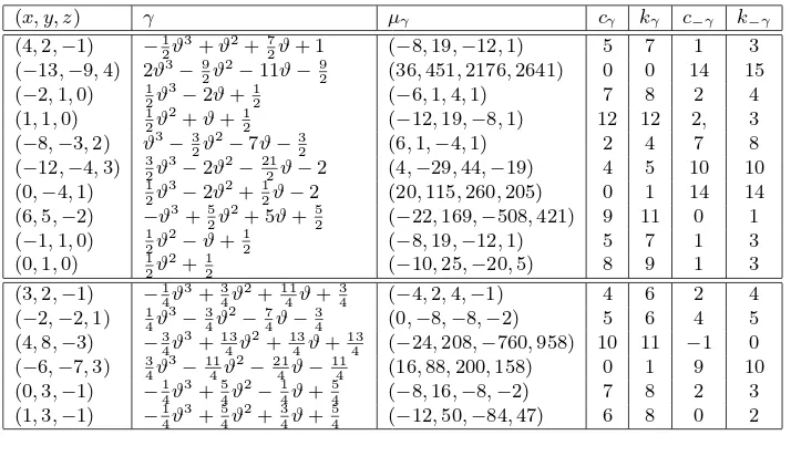
(1) t= 2, γ=x·ϑ+y·1+ϑ2
From here on we proceed as in the proof of Theorem 5.3. The details of the computation are given in Table 3 below where we use the following notation: (x, y, z) denote the coordinates of γ as in the table above, the minimal polynomial µγ =X4+a1X3+a2X2+a3X+a4 of γ is given by
Power integral bases in the polynomial orderZ[α] ofKt were described
by G. Lettl and A. Peth˝o [22].
Theorem 5.3. Let t∈N\ {0,3} andϑ denote a root of the polynomial
Then we haveF0(Q(ϑ)) =∅ and F1(Q(ϑ)) =G ∪ G1∪ G2∪ G4 where
G=
{−3−ϑ,−t−2 +ϑ,−2−6ϑ−tϑ2+ϑ3,−t−3 + 6ϑ+tϑ2−ϑ3},
if t≥5,
∅ otherwise,
G1 =
{−4 +ϑ,−4−ϑ,−5 + 6ϑ+ϑ2−ϑ3,−3−6ϑ−ϑ2+ϑ3, −23 + 3ϑ2−ϑ3,−1−3ϑ2+ϑ3,−14 + 25ϑ+ 2ϑ2−4ϑ3,
−10−25ϑ−2ϑ2+ 4ϑ3}, if t= 1,
∅ otherwise,
G2 =
{−5 +ϑ,−3−ϑ,−5 + 6ϑ+ 2ϑ2−ϑ3,−3−6ϑ−2ϑ2+ϑ3},
if t= 2,
∅ otherwise,
G4 =
{−6 +ϑ,−3−ϑ,1 + 9ϑ−22ϑ2+ 4ϑ3,−78−9ϑ+ 22ϑ2−4ϑ3,
−7 + 6ϑ+ 4ϑ2−ϑ3,−3−6ϑ−4ϑ2+ϑ3,−62 + 74ϑ+ 30ϑ2−9ϑ3, −15−74ϑ−30ϑ2+ 9ϑ3}, if t= 4,
∅ otherwise.
Before embarking on the proof of Theorem 5.3 we need some preparation. For checking the CNS property of some polynomials we exploit a technical lemma.
Lemma 5.1. The polynomial X4+p3X3+p2X2+p1X+p0∈Z[X] with
the properties
(i) p0 ≥4 (ii) p1 ≥p0+ 1 (iii) p3 ≥2 (iv) p1 ≥2p2+ 1
(v) 2p1−p2+ 2p3 ≤2p0−1
is a CNS polynomial.
Proof. Let
E={(e1, . . . , e4)∈Z4| |ei| ≤2 (i= 1, . . . ,4), (e2, e1)6= (0,±2),
eiei+1 ≤0 (i= 1,2,3), |ei|= 2 =⇒ ei−1= 06 (i= 2,3,4)} and τP(A) be the mapping defined in Section 2. Clearly, property (i) of
several steps thereby using the notation of ([26], Lemma 1): a−→(S) indicates thatτP(A) falls into step(s)S considered before.
(1)e4≥0, τP(0,0,0, e4) = 0
This concludes the proof.
We are now in a position to verify Theorem 5.3.
Proof of Theorem 5.3. By [9] up to equivalence all generators of power integral bases ofZ[ϑ] are the following:
• fort= 1 additionally: 3ϑ2−ϑ3,25ϑ+ 2ϑ2−4ϑ3,
• fort= 4 additionally: 9ϑ−22ϑ2+ 4ϑ3,−74ϑ−30ϑ2+ 9ϑ3.
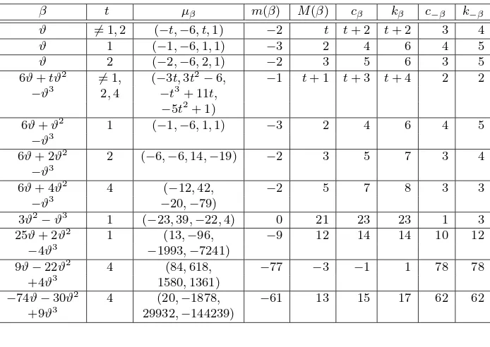
We proceed analogously as in the proof of Theorem 3.3 by using Proposition 2.1 and Table 4 below with the following notation: β is a generator of a power integral basis ofQ(ϑ). The minimal polynomialµβ =X4+a1X3+
a2X2+a3X+a4 ofβ is listed in the form (a1, a2, a3, a4). Lower bounds for the constants cβ, kβ are given by Proposition 2.1. For their determination
([3], Theorem 3.1) and Corollary 5.1 are used in a straightforward way. Similarly as in the proof of Theorem 3.3 Remark 2 is used. ✷
β t µβ m(β) M(β) cβ kβ c−β k−β
ϑ 6= 1,2 (−t,−6, t,1) −2 t t+ 2 t+ 2 3 4 ϑ 1 (−1,−6,1,1) −3 2 4 6 4 5 ϑ 2 (−2,−6,2,1) −2 3 5 6 3 5 6ϑ+tϑ2
6
= 1, (−3t,3t2
−6, −1 t+ 1 t+ 3 t+ 4 2 2
−ϑ3
2,4 −t3
+ 11t,
−5t2
+ 1) 6ϑ+ϑ2
1 (−1,−6,1,1) −3 2 4 6 4 5
−ϑ3 6ϑ+ 2ϑ2
2 (−6,−6,14,−19) −2 3 5 7 3 4
−ϑ3
6ϑ+ 4ϑ2
4 (−12,42, −2 5 7 8 3 3
−ϑ3 −20,−79)
3ϑ2
−ϑ3 1 (−23,39,−22,4) 0 21 23 23 1 3
25ϑ+ 2ϑ2
1 (13,−96, −9 12 14 14 10 12
−4ϑ3
−1993,−7241) 9ϑ−22ϑ2
4 (84,618, −77 −3 −1 1 78 78
+4ϑ3
1580,1361)
−74ϑ−30ϑ2
4 (20,−1878, −61 13 15 17 62 62
+9ϑ3
29932,−144239)
Table 4
Finally we consider another family of orders in a parametrized family of quartic number fields, where all power integral bases are known. Lett∈Z,
t≥0, and P(X) =X4−tX3−X2+tX+ 1. Denote byα one of the zeros ofP(X). In the following we deal with the order O=Z[α] of Q(α).
M. Mignotte, A. Peth˝o and R. Roth [23] gave the following result:
Theorem 5.4. (M. Mignotte, A. Peth˝o, R. Roth) Let t≥4. Then every element γ ∈ O such that Z[γ] = O is equivalent to some element
γ =xα+yα2+zα3 with
(x, y, z)∈ {(1,0,0),(1, t,−1),(t, t−1,−1),(t,−t−1,1),(1,0,−1),
except when t = 4, in which case additionally (x, y, z) ∈ {(209,140,−49),
(209,−312,64)}. 1
Theorem 5.5. Let t≥4. We haveF0(Q(α)) =∅ andF1(Q(α)) =G4∪ Gt
where
G4=
209α+ 140α2−49α3+ 350,209α−312α2+ 64α3−71 Gt=
α+t+ 1, α+tα2−α3+t+ 2, tα+ (t−1)α2−α3+ 8,
tα−(t+ 1)α2+α3+ 2, α−α3+ 2, α−t(t2+ 1)α2+t2α3−t+ 1 .
Proof. We follow the same line as in the proof of Theorem 5.3. First we compute the data necessary to apply Algorithm 2.1. For the zeroes of the polynomialP(X) we use the following estimates:
α1 =t−1/t3−1/t5−4/t7−9/t9, α2=−1/t−1/t5−1/t7−5/t9,
α3 = 1 + 1/2t+ 1/8t2+ 1/2t3, α4=−1 + 1/2t−1/8t2.
In a straightforward way we obtainM(γ) for any possible value ofγ. Know-ing M(γ) it is easy to establish kγ. Because of the special form of P(X)
we do not needk−γ. Indeed denote byσ the automorphism ofQ(α), which
maps α to−α1. Then an easy computation shows that
σ(−α) =α+tα2−α3−t σ(−(tα+ (t−1)α2−α3)) =tα−(t−1)α2+α3+ 1
σ(−(α−α3)) =α−t(t2+ 1)α2+t2α3+t3
and if t= 4 then
σ(−(209α+ 140α2−49α3)) = 209α−312α2+ 64α3+ 116.
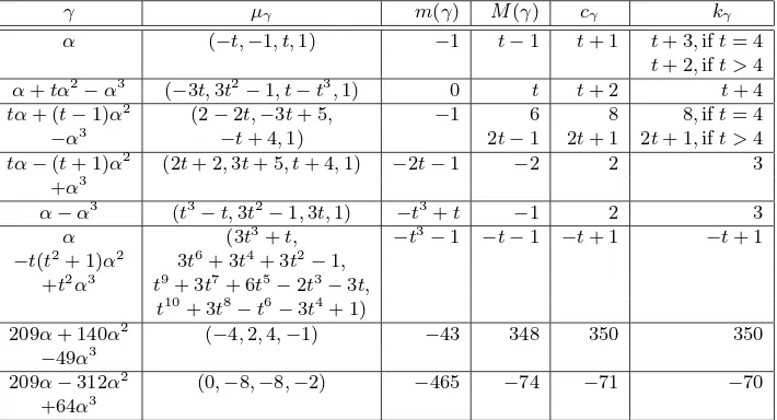
The details of the computation are given in Table 5 below where we use the following notation: (x, y, z) denote the coordinates ofγ=xα+yα2+zα3 as in Theorem 5.4, the minimal polynomialµγ=X4+a1X3+a2X2+a3X+a4 ofγ is given by (a1, a2, a3, a4).
By the intention of the journal we had to omit further details of the proof, because it is quite complicated and long especially in the caseγ =α+
tα2−α3. The interested reader may find the complete version electronically under the URL:
http://www.inf.unideb.hu/˜pethoe/Publications.html.
γ µγ m(γ) M(γ) cγ kγ eralization of the radix representation – a survey, in ”High Primes and Misdemeanours: lectures in honour of the 60th birthday of Hugh Cowie Williams”, Fields Institute Commu-cations, vol.41(2004), 19–27.
[2] S. Akiyama, T. Borb´ely, H. Brunotte, A. Peth˝oandJ. M. Thuswaldner,Generalized radix representations and dynamical systems I, Acta Math. Hung.,108(2005), 207–238. [3] S. Akiyama, H. BrunotteandA. Peth˝o,Cubic CNS polynomials, notes on a conjecture
of W.J. Gilbert, J. Math. Anal. and Appl.,281(2003), 402–415.
[4] S. Akiyama and H. Rao, New criteria for canonical number systems, Acta Arith.,111 (2004), 5–25.
[5] S. AkiyamaandJ. M. Thuswaldner,On the topological structure of fractal tilings gener-ated by quadratic number systems, Comput. Math. Appl.49(2005), no. 9-10, 1439–1485. [6] T. Borb´ely,Altal´´ anos´ıtott sz´amrendszerek, Master Thesis, University of Debrecen, 2003. [7] H. Brunotte,On trinomial bases of radix representations of algebraic integers, Acta Sci.
Math. (Szeged),67(2001), 521–527.
[8] H. Brunotte,On cubic CNS polynomials with three real roots, Acta Sci. Math. (Szeged), 70(2004), 495 – 504.
[9] I. Ga´al,Diophantine equations and power integral bases, Birkh¨auser (Berlin), (2002). [10] W. J. Gilbert,Radix representations of quadratic fields, J. Math. Anal. Appl.,83(1981),
264–274.
[11] E. H. Grossman,Number bases in quadratic fields, Studia Sci. Math. Hungar.,20(1985), 55–58.
[12] V. Gr¨unwald,Intorno all’aritmetica dei sistemi numerici a base negativa con particolare riguardo al sistema numerico a base negativo-decimale per lo studio delle sue analogie coll’aritmetica ordinaria (decimale), Giornale di matematiche di Battaglini,23(1885), 203– 221, 367.
[14] I. K´atai and B. Kov´acs, Kanonische Zahlensysteme in der Theorie der quadratischen algebraischen Zahlen, Acta Sci. Math. (Szeged),42(1980), 99–107.
[15] I. K´ataiandB. Kov´acs,Canonical number systems in imaginary quadratic fields, Acta Math. Acad. Sci. Hungar.,37(1981), 159–164.
[16] I. K´ataiand J. Szab´o,Canonical number systems for complex integers, Acta Sci. Math. (Szeged),37(1975), 255–260.
[17] D. E. Knuth,An imaginary number system, Comm. ACM,3(1960), 245 – 247.
[18] D. E. Knuth, The Art of Computer Programming, Vol. 2 Semi-numerical Algorithms, Addison Wesley (1998), London 3rd edition.
[19] B. Kov´acs,Canonical number systems in algebraic number fields, Acta Math. Acad. Sci. Hungar.,37(1981), 405–407.
[20] B. Kov´acs and A. Peth˝o,Number systems in integral domains, especially in orders of algebraic number fields,Acta Sci. Math. (Szeged),55(1991), 287–299.
[21] S. K¨ormendi,Canonical number systems inQ(√3
2),Acta Sci. Math. (Szeged),50(1986), 351–357.
[22] G. Lettland A. Peth˝o,Complete solution of a family of quartic Thue equations, Abh. Math. Sem. Univ. Hamburg65(1995), 365–383.
[23] M. Mignotte, A. Peth˝oandR. Roth,Complete solutions of quartic Thue and index form equations,Math. Comp.65(1996), 341–354.
[24] P. Olajos,Power integral bases in the family of simplest quartic fields, Experiment. Math. 14(2005), 129–132.
[25] A. Peth˝o,On a polynomial transformation and its application to the construction of a public key cryptosystem, Computational Number Theory, Proc., Walter de Gruyter Publ. Comp. Eds.: A. Peth˝o, M. Pohst, H. G. Zimmer and H. C. Williams (1991), 31–43. [26] A. Peth˝o,Notes on CNS polynomials and integral interpolation, More sets, graphs and
numbers, 301–315, Bolyai Soc. Math. Stud., 15, Springer, Berlin, 2006.
[27] A. Peth˝o, Connections between power integral bases and radix representations in alge-braic number fields, Proc. of the 2003 Nagoya Conf. ”Yokoi-Chowla Conjecture and Related Problems”, Furukawa Total Pr. Co. (2004), 115–125.
[28] R. Robertson,Power bases for cyclotomic integer rings, J. Number Theory,69(1998), 98–118.
[29] R. Robertson,Power bases for 2-power cyclotomic integer rings, J. Number Theory,88 (2001), 196–209.
[30] K. Scheicher,Kanonische Ziffernsysteme und Automaten,Grazer Math. Ber.,333(1997), 1–17.
[31] D. Shanks,The simplest cubic fields,Math. Comp.,28(1974), 1137–1152.
HorstBrunotte
Universit´e Gauss Haus-Endt-Straße 88 D-40593 D¨usseldorf, Germany
E-mail:[email protected]
AndreaHuszti
Faculty of Informatics University of Debrecen
P.O. Box 12, H-4010 Debrecen, Hungary
Hungarian Academy of Sciences and University of Debrecen
E-mail:[email protected]
AttilaPeth˝o
Faculty of Informatics University of Debrecen
P.O. Box 12, H-4010 Debrecen, Hungary
Hungarian Academy of Sciences and University of Debrecen
E-mail:[email protected]