Full Terms & Conditions of access and use can be found at
http://www.tandfonline.com/action/journalInformation?journalCode=ubes20
Download by: [Universitas Maritim Raja Ali Haji] Date: 12 January 2016, At: 17:19
Journal of Business & Economic Statistics
ISSN: 0735-0015 (Print) 1537-2707 (Online) Journal homepage: http://www.tandfonline.com/loi/ubes20
Reform of Unemployment Compensation in
Germany: A Nonparametric Bounds Analysis Using
Register Data
Sokbae Lee & Ralf A. Wilke
To cite this article: Sokbae Lee & Ralf A. Wilke (2009) Reform of Unemployment Compensation in Germany: A Nonparametric Bounds Analysis Using Register Data, Journal of Business & Economic Statistics, 27:2, 193-205, DOI: 10.1198/jbes.2009.0014
To link to this article: http://dx.doi.org/10.1198/jbes.2009.0014
Published online: 01 Jan 2012.
Submit your article to this journal
Article views: 98
Reform of Unemployment Compensation in
Germany: A Nonparametric Bounds Analysis
Using Register Data
Sokbae L
EEInstitute for Fiscal Studies and University College London, London, UK (l.simon@ucl.ac.uk)
Ralf A. W
ILKEUniversity of Nottingham, University Park, Nottingham NG7 2RD, UK (ralf.wilke@nottingham.ac.uk)
Economic theory suggests that an extension of the maximum length of entitlement for unemployment benefits increases the duration of unemployment. Empirical results for the reform of the unemployment compensation system in Germany during the 1980s are less clear. The analysis in this article is motivated by recent developments in econometrics for partial identification. We use extensive administrative data with the drawback that we can only observe lower and upper bounds for the true unemployment duration. For this reason we bound the reform effect on unemployment duration taking account of the fact that observed unemployment spells are only interval data. We identify a systematic increase in unemployment duration in response to the reform in samples that amount to about 10% of the unemployment spells for the treatment group.
KEY WORDS: Interval data; Nonparametric bounds analysis; Partial identification; Treatment effect; Unemployment duration.
1. INTRODUCTION
Many empirical contributions consider the question whether unemployment durations increase with the entitlement length for unemployment benefits. This is suggested by economic theory, which also predicts an increase with the level of the unemployment compensation. See Katz and Meyer (1990) for a summary. Some empirical evidence for this is observed for the United States (Katz and Meyer 1990) and for the United Kingdom (van den Berg 1990).
In Germany, the maximum entitlement length for unem-ployment benefits for older employees was increased from 12 months initially to up to 32 months during the 1980s. This article analyzes the effect of this reform on unemployment durations. The analysis of the reform of the 1980s is highly relevant for the current German economy, because recent labor market reforms, which came into force in 2006, basically withdrew the former reform and reduced maximum entitlement periods for unemployment benefits. The reform of the 1980s presents a unique opportunity to identify the effect of an increase in the maximum entitlement length in a natural experiment setup because, by the nature of law changes, the reform only affects some age groups (42 years old and older) of the population. It was already subject to several empirical investigations (see, for example, Biewen and Wilke 2005, for a summary).
The only clearcut finding to date is that it was creating the conditions for massive early retirement at the expense of the unemployment insurance system. Both employers and older employees agreed to early retirement packages, thus negating the greater dismissal protection for older employees with long-term company affiliation (Fitzenberger and Wilke 2010). However, the results are less clear when one focuses on the group of older unemployed persons who have not taken early retirement (i.e., those who are still looking for new jobs).
There exist two types of data available for the study of German unemployment: household survey data called the German Socio-Economic Panel (GSOEP) and register data called the IAB employment subsample (IABS). Empirical studies using GSOEP do not have conclusive findings (see Table 1 for a selective summary or see Plaßmann 2002, table 16 for more details). Schneider and Hujer (1997) do not find increases in unemployment duration, whereas Hunt (1995) and Hujer and Schneider (1995) report such increases for some age groups of males. The differences in the results may be driven by differences in the samples used or by different econometric models. Compared with the GSOEP, the IABS is a much larger sample and therefore one may obtain more accurate estimates using the IABS than the GSOEP. However, one main problem with the IABS is that one can only observe lower and upper bounds for the true unemployment duration. Using register data, Plaßmann (2002) finds strong effects, but her econometric framework does not take into account that the true unem-ployment period is only partially identified. Fitzenberger and Wilke (2010) point to the problem of measuring unemployment spells error and obtain rather different estimation results for two different proxies for unemployment in the data. In par-ticular, using nonparametric techniques they find that unem-ployment durations of those who reenter emunem-ployment did not seem to increase in response to the reform, whereas the share of exits from unemployment to out of the labor force increased dramatically. Although their econometric approach for the identification of the treatment effect is nonparametric, their results may be affected by different sample compositions for the two unemployment definitions.
193
2009 American Statistical Association Journal of Business & Economic Statistics April 2009, Vol. 27, No. 2 DOI 10.1198/jbes.2009.0014
In an attempt to reconcile different results in the literature, Biewen and Wilke (2005) apply several duration models to both survey and register data from the same period and with the same set of regressors. The resulting coefficients for long entitlement periods are generally not statistically significant in the case of the survey data. In contrast, there are sharp results patterns with the register data. Their results suggest that one should look at the register data given the large sample size of the IABS. Because their models applied (and also the models in the other con-tributions) are not appropriately specified for the identification of the reform effect using the IABS, they conclude that further research is necessary that uses better adapted econometric models. The analysis in this article is motivated by these ambiguous empirical findings and by recent developments in econometrics for partial identification. As noted earlier, in the IABS data, for many individuals, one can only observe lower and upper bounds for the unemployment duration. As a result, without imposing untenable assumptions on the data-generating pro-cess, it would be only possible to identify the effect of the reform up to a set. However, this type of set identification or partial identification can bring consensus among empirical research-ers, because empirical results based on partial identification can be regarded as more credible findings.
We aim to gain robust insights into the extent to which the conducted reform in West Germany has increased unemployment spells using register-based data. We identify a systematic increase in unemployment duration in response to the reform in samples that amount to about 10% of the unemployment spells for the treatment group. This share is small for the following main rea-son: In this article we obtain that for about 50% of the unem-ployment spells, the actual entitlement length for unemunem-ployment benefits is shorter than the maximum entitlement length. This implies that many older unemployed persons were in fact not treated at all by the reform or their treatment was smaller than the maximum extension of the entitlement length. All past articles in this field do not exclude these spells from their analysis, which may also explain the lack of statistical significance in many cases. The article is organized as follows. Section 2 provides a brief description of the reform and data. Section 3 describes our estimation strategy and Section 4 discusses our empirical findings. Section 5 concludes.
2. INSTITUTIONAL FRAMEWORK AND DATA
In Germany, an unemployed person with a sufficient amount of working experience is entitled to unemployment benefits.
The length of the entitlement period depends on the length of the employment periods before the beginning of the unem-ployment period and on the age of the unemployed person. The maximum entitlement length for unemployment benefits for unemployed persons age 42 years or older was increased dur-ing the years 1985–1987. A detailed description of the German unemployment compensation system and changes in unem-ployment compensation laws can be found, for example, in Hunt (1995) and Plaßmann (2002).
Until 1984, 12 months of compensation was allotted for all unemployed persons. After 1987, the maximum entitlement length was 18 months for unemployed persons age 42 to 43 years, 22 months for unemployed persons age 44 to 48 years, 26 months for unemployed persons age 49 to 53 years, and 32 months for unemployed persons age 54 years and older. See Hunt (1995, tables 1 and 2) for an overview.
After exhaustion of unemployment benefits, unemployed persons generally drew unemployment assistance that was granted on an annual basis without any maximum period. Unemployment assistance was merged with social benefits and was replaced by a new system of social benefits in 2005, which implies that the institutional setting after expiration of unem-ployment benefits nowadays differs from the system in the 1980s. For our analysis we classify the calendar years 1981– 1988 into three categories because the reform was conducted over a 3-year period:
1. Prereform period: 1981–1983 2. Reform period: 1984–1986 3. Postreform period: 1987–1988
Year 1984 is considered a reform year because unemploy-ment spells starting in 1983 are the latest not affected at all by the reform. The entitlement length in many spells starting in 1984 was extended in 1985 after the reform came into force. Anticipation behavior in 1984 may also affect our estimation results. Years before 1981 are not considered because of data quality issues. For example, the information on transfer pay-ments seems to be incomplete in the data, see Bender et al. (1996) for details. As postreform years, we use 1987–1988 (2 years). Year 1987 is included because the postreform system already applies to most of the unemployment spells starting in 1987. Years after 1988 are not considered because of the sys-tematic changes in labor market conditions during and after German unification.
It is also important to note that the extension of the maximum entitlement lengths has different implications for
Table 1. Summary of selected empirical results
Source Data Effect of the entitlement period for unemployment benefits Hunt (1995) GSOEP 1983–1988 Significant increase in unemployment duration for males age 44–48 years Hujer and Schneider (1995) GSOEP 1983–1992 Significant increase in unemployment duration for males only
Schneider and Hujer (1997) GSOEP 1992–1993 No significant effect on unemployment duration Plaßmann (2002) IABS 1982–1995 Significant effect on unemployment duration
Fitzenberger and Wilke (2010) IABS 1981–1997 Increase in unemployment duration with exits to out of the labor market; no apparent increase in job search periods
Biewen and Wilke (2005) GSOEP 1983–1997 No significant effect on unemployment duration
IABS 1983–1997 Significant positive relation with unemployment duration for males only
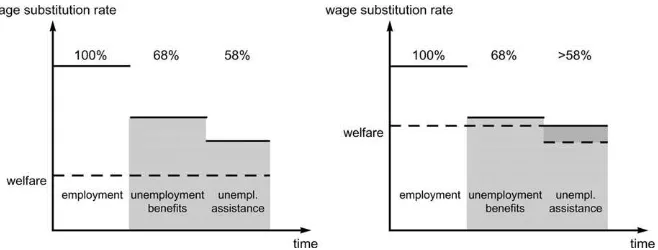
unemployed persons depending on the levels of income transfers during the unemployment duration. In particular, it matters most for individuals with high preunemployment earnings. The wage replacement rate for unemployment ben-efits (unemployment assistance) depends on previous earnings. In addition, unemployment assistance is means tested (i.e., it decreases with the income generated by other household members and, in some cases, it depends on expected earnings). Unemployed persons with low preunemployment income may therefore obtain social benefits as additional income transfers if the level of unemployment benefits (unemployment assistance) is below the welfare level. This is the case if income transfers from the employment offices are not high enough to cover the basic needs of the household. Households (and not individuals) are eligible for social benefits, which are means tested and the level depends mainly on the municipality and on the demo-graphic structure of the household. See Wilke (2006) for more details about the social benefits system in Germany until 2004. Any form of social benefits is paid by the German munici-palities. If transfers from the employment office plus other household income is less than this level, the household is entitled to welfare support. The reform should therefore have a smaller effect on those with low preunemployment earnings, because an increase in unemployment compensation would simultaneously decrease the level of additional social benefits, resulting in a zero or very small net change. See Figure 1 (right). The same reasoning applies to individuals with high former income levels for which we expect a greater increase in income transfers after the reform (see Fig. 1, left). We may therefore expect stronger reform effects for this group.
To summarize, the reform under consideration implies an increase of the unemployment compensation level between 12 months of unemployment duration and the new maximum entitlement length; the net increase may differ depending on the level of preunemployment earnings. Unfortunately, we observe neither the level of unemployment compensation paid by the employment offices nor social benefits transfers from the municipalities, which leaves us the preunemployment earnings and the type of income transfers from the employment offices as the only observable determinants for the wage replacement rate. The wage replacement rate also depends on whether the claimant has dependent children. Information about children is unreliable in our data and not available at all before 1983. For this reason we decided to ignore it in the
analysis. Therefore, we construct dummy variables indicating whether the preunemployment wage is located in the bottom (top) three (two) quintiles of the IABS population income distribution of full-time employees in the year when the unemployment spells begins. The bottom (top) quintiles are referred to as low (high) preunemployment earnings in this article. To ensure that our sample has, indeed, long entitlement periods for unemployment benefits, we will only consider unemployment with a long-term employment period before unemployment.
We use individuals age 36 to 41 years as the control group in our analysis. These are the oldest individuals not affected by the reform. We select the individuals age 44 to 48 years as the treatment group. This is done for the following reasons: Those age 42 to 43 are excluded because the short extension of the maximum entitlement length to 18 months implies a weak treatment of this group. Persons older than 48 years are not considered because Fitzenberger and Wilke (2010) find there is already some evidence that early retirement starts within the age group 49 to 53 and we want to focus our analysis on individuals still looking for jobs. During the reform under consideration, the maximum entitlement length for unem-ployment benefits increased from 12 to 22 months for the treatment group, whereas it remained constant for the control group. A comprehensive summary of the institutional setting and the changes in the German unemployment compensation system can be found in Hunt (1995) and Plaßmann (2002). Further details are therefore not presented here.
For our estimations we use the IABS 1975–1997, which contains daily information about employment periods that have been subject to social insurance payments of about 500,000 individuals in West Germany. The data are a representative 1% sample of the workforce in Germany during the whole period 1975–1997. It provides daily information about the labor market status of the individuals during a period of more than 20 years. For a general description of the data, see Bender, Haas, and Klose (2000). General advantages of these data are the large sample size and the daily register-based records, which are likely to be more precise than household interview-based data. A disadvantages of the IABS are the small number of observed variables and the missing information about parts of an unemployment period, because only information about the receipt of unemployment compensation from the German federal labor office is observed. Until 2004, these were
Figure 1. The level of income transfers in Germany is never below the welfare level. Example for high (left) and low (right) preunemployment wages (when there are children involved).
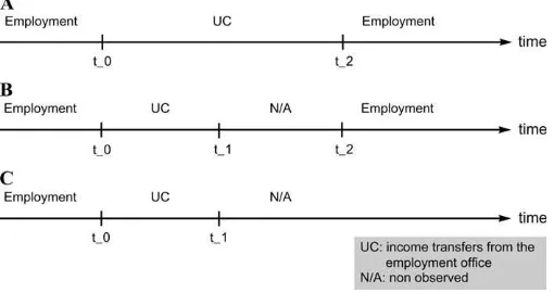
unemployment benefits (UB, Arbeitslosengeld; Hunt 1995) refers to this as unemployment insurance, ALG), unemploy-ment assistance (UA, Arbeitslosenhilfe; Hunt (1995) uses the abbreviation ALH), or income maintenance during further training (IMT, Unterhaltsgeld). Periods of unemployment without the receipt of unemployment compensation or the receipt of social benefits from the municipalities are not recorded in the data. In addition, there is no information about periods of self-employment, and lifetime civil servants are also not included in the data. This implies that unobserved periods may correspond either to unemployment, self-employment, or out-of-labor-force status (see Fig. 2 for an illustration that pres-ents three common samples of the data structure). Fitzenberger and Wilke (2010) address this problem of measurement error and proxy unemployment with two definitions. They introduce the nonemployment (NE) proxy as an upper bound for the unemployment duration and the unemployment between jobs (UBJ) proxy as a lower bound. In their sensitivity-type analy-sis, it is evident that the results strongly depend on the defi-nition of unemployment.
The analysis in this article intends to bound the effect of the reform of the unemployment compensation system over the natural lower and upper bounds of the true unemployment period that can be extracted from the data. For this purpose we use the NE proxy of Fitzenberger and Wilke (2010) as the upper bound:
Nonemployment (NE): all periods of nonemployment after an employment period that contain at least one period with income transfers by the German federal labor office. The nonemployment period is considered as censored if the last record involves a UB, UA, or IMT payment that is not followed by an employment spell. A nonemployment spell is treated as right censored if it is not fully observed.
With this definition of unemployment, we include periods that are not explicitly recorded in the data (out of the labor force, social benefits). In this case we do not know whether the individual is still unemployed, out of the labor force, or self-employed. This seems to be a natural approach, because we cannot distinguish unemployment spells from periods of out of the labor market. It is therefore an upward-biased proxy of the true unemployment duration. We now consider a proxy for the lower bound of unemployment duration:
Unemployment with permanent income transfers(UPIT): all periods of nonemployment after an employment period with a continuous flow of unemployment compensation from the German federal labor office. Maximum interruption in com-pensation transfers is 1 month; in the case of cutoff times, 6 weeks. An observation is marked as right censored at the last day of the duration before the transfers are interrupted for more than 1 month or in the event of there being no observation after the last compensation transfer.
We introduce the UPIT proxy because the UBJ proxy of Fitzenberger and Wilke (2010) may be too narrow for our purposes. This is mainly because the latter conditions on the future exit to employment. This is a valuable property for the identification of the increase in early retirement as undertaken by Fitzenberger and Wilke (2010), but in our analysis we may lose too much information—in particular, for all individuals who no longer enter employment. This may prevent us from obtaining tight bounds for the treatment effect. In general, we have UPIT#NE.
Let us illustrate the difference between UPIT and NE with the help of Figure 2. In case A, all proxies yield the same length for the unemployment duration: UPIT¼NE¼t2–t0. In case B
we obtain UPIT¼t1–t0(right censored) and NE¼t2–t0if the
length of the nonobserved period is greater than 1 month; otherwise, we obtain case A. In case C we have UPIT¼NE¼ t1–t0(right censored). There is another important difference
between the construction of our samples and the samples used in Fitzenberger and Wilke (2010). The latter extract samples of different size for their estimations. Their estimates may therefore be affected by sample selection issues, which are not present in our approach because we compute the lower and upper bounds for each unemployment duration in the same sample.
For our empirical analysis we restrict the sample of unem-ployment periods to males because effects of the reform on females may be distorted by other factors such as introduction of parental leave benefits and upward trends of labor force participation of females. The sample was further refined by selecting an additional number of observable characteristics of the unemployed. This is done because we aim to ensure that the included unemployed persons indeed have a certain length of entitlement for unemployment benefits at the beginning of the current unemployment period. For this reason we do not include unemployment periods that are likely related to seasonal unemployment and temporary layoffs. We do not impose restrictions on the educational degree because, in our analysis for given wage level, we find similar results for educational groups. For this reason we use a pooled sample. In particular we restrict our sample to
d Unemployment periods with unemployment benefits as
the first observed income transfer payment
d No receipt of any unemployment transfer during the past
12 months before the current unemployment period
d No recall to the former employer after the last
unem-ployment period
d Exclude the business sector of ‘‘agriculture’’ (last
employment)
Figure 2. Three common examples of the data structure.
We only consider unemployment periods starting with unemployment benefits as first income transfer because we aim at investigating a reform of the system of unemployment benefits. Unfortunately, we do not observe the actual entitle-ment length for unemployentitle-ment benefits in the data, and a construction of such a variable is complicated because it has to be computed for each individual work history, which consists of up to 100 records in the data. This is laborious because many individuals have periods of nonemployment or unemployment between their employment periods, which implies that the actual entitlement length for unemployment benefits does not immediately follow from the length of the last employment period. For this reason we use the simple rule that unemployed persons did not receive any unemployment compensation within the year prior to unemployment and that they were generating entitlements during this time. This does not ensure that the unemployed persons actually do have maximum enti-tlement for unemployment compensation, but we found that the median length of employment before unemployment is more than 3 years after the reform. This would imply a median entitlement length of more than 18 months for the treatment group after the reform. The inclusion of individuals with shorter entitlement lengths implies that, for some observations in the sample, the reform should only affect a shorter part of the unemployment duration. For this reason our estimation results between months 12 and 22 of the unemployment duration maybe downward biased. The bias increases as we step closer to month 22, because less individuals got the maximum treat-ment than a small extension of the entitletreat-ment length. At the same time there are fewer individuals getting the maximum
treatment, which implies that the overall impact of the reform might be smaller than the size of our sample suggests.
Tables 2 and 3 present the summary statistics for the pre- and postreform samples that are used for the estimations. These reported summary statistics are for married males, because this is the population used for most of the empirical analysis. In total we have 4,049 unemployment spells in our sample, of which 2,922 (72%) are recorded during the prereform period. By definition, the length of UPIT is shorter than that of NE. We observe that the average length of NE periods is about twice the length of UPIT periods. About 70% of the UPIT spells have the same length as the NE spells. On one hand, using the median spell length of UPIT, the difference-in-differences (DID) estimate of the effect of the reform is 5 days. On the other hand, using the median spell of NE, the estimate for the same effect is 84 days. Hence, just by looking at these back-of-the-envelope cal-culations, one may expect that the reform effect possibly varies across the unemployment proxies, which motivates our analysis.
3. ECONOMETRIC FRAMEWORK
3.1 Bounds Analysis for Treatment Effects
This section describes an econometric approach used in the article. Our framework is based on bounds analysis (see a monograph by Manski (2003) for a review). In particular, we present bounds for treatment effects in the context of DID. We also obtain tighter bounds using some plausible independence and monotonicity assumptions. See, for example, Manski and Pepper (2000) and Blundell et al. (2007) for implications of
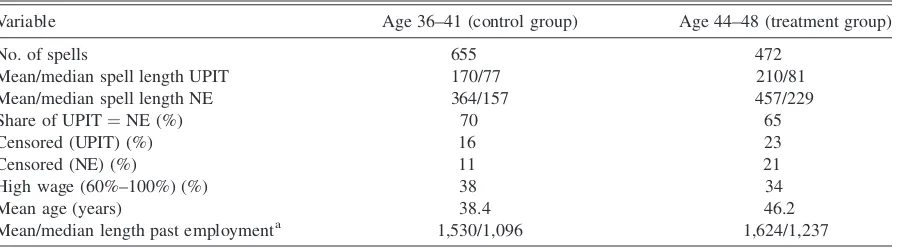
Table 3. Descriptive summary of the sample: Postreform years (married males)
Variable Age 36–41 (control group) Age 44–48 (treatment group)
No. of spells 655 472
Mean/median spell length UPIT 170/77 210/81 Mean/median spell length NE 364/157 457/229 Share of UPIT¼NE (%) 70 65
Censored (UPIT) (%) 16 23
Censored (NE) (%) 11 21
High wage (60%–100%) (%) 38 34
Mean age (years) 38.4 46.2
Mean/median length past employmenta 1,530/1,096 1,624/1,237
NOTE: aComputed from left-censored data and ignores information before first January 1980.
Table 2. Descriptive summary of the sample: Prereform years (married males)
Variable Age 36–41 (control group) Age 44–48 (treatment group)
No. of spells 1,581 1,341
Mean/median spell length UPIT 193/92 207/91 Mean/median spell length NE 450/163 407/151 Share of UPIT¼NE (%) 71 75
Censored (UPIT) (%) 19 20
Censored (NE) (%) 13 16
High wage (60%–100%) (%) 34 32
Mean age (years) 38.6 45.8
Mean/median length past employmenta 1,074/761 1,150/852 NOTE: aComputed from left-censored data and ignores information before first January 1980.
imposing some credible assumptions. There are no new ideas in our econometric framework; however, details of bounds anal-ysis are newly developed to analyze DID-type treatment effects under a natural experiment. See Manski and Tamer (2002) for inference on regressions with interval data. See Honore´ and Lleras-Muney (2006) for an application of bounds analysis to duration analysis in the context of competing risks models. See also Manski (1990, 1997) and Lechner (1999) for non-parametric bounds of treatment effects.
To describe our econometric model, assume that we observe interval data on the duration variable of interest—say,Y. That is, we observeY1andY2, whereY1#Y2, and it is only known
that latent durationYis betweenY1andY2. For example, ifY1¼ Y2, then observed duration is a point and equal toY; however, in
general, if we haveY1<Y2, thenYis in the interval betweenY1
andY2. In our application,Yis the unemployment spell,Y1is
UPIT, andY2is NE.
We consider two types of treatment effects: one on the sur-vival probability ofYand the other on the quantiles ofY con-ditional on explanatory variablesX. For simplicity, we assume thatXis a vector of discrete random variables. Both treatment effects are defined as DID in terms of survival probability and quantiles, respectively. It is plausible that the DID estimates can be regarded as treatment effects because the reform we consider can be thought of as a natural experiment.
First we present bounds for the treatment effects in terms of survival probability. To do so, letPdenote time periodspt0and pt1(before and after a treatment) andTdenote age groups 0 and
1 (control and treatment groups). In our application, pt0 ¼
1981, 1982, 1983 and pt1 ¼ 1987, 1988. Also, age group 0
consists of individuals age 36 to 41 years and age group 1 is composed of individuals age 44 to 48 years. We define the effect of a reform to be
Dðyjx;pt0;pt1Þ ¼ ½Sðyj1;pt1;xÞ Sðyj0;pt1;xÞ
½Sðyj1;pt0;xÞ Sðyj0;pt0;xÞ; ð1Þ
whereS(y|t,p,x)¼P(Y>y|T¼t,P¼p,X¼x). The effect of the reform defined in Equation (1) can be viewed as a non-parametric specification of the treatment effect on the treated, provided that the survivor probabilities of treated and controls would have followed parallel paths without the reform. See assumption 3.1 and equation (9) of Abadie (2005) for a general description of the nonparametric identification of DID models. In our empirical application, this is reasonable to assume that unemployed persons age 44 to 48 years (treatment group) and unemployed persons age 36 to 41 years (control group) would have had parallel paths without the reform, because both groups are more or less in the same life cycle stage and the conducted reform is mainly based on the age of the unemployed person.
IfYwere observed, then the treatment effect could be esti-mated by a sample analog to Equation (1). Obviously, this is unfeasible because we have only interval data onY. A natural approach is to boundD(y|x,pt0,pt1) by combining bounds for
four survival probabilities.
DefineS1(y|t,p,x)¼P(Y1>y|T¼t,P¼p,X¼x) andS2(y|t, p, x) ¼ P(Y2 > y|T ¼ t, P ¼ p, X ¼ x). Without imposing
additional conditions, then the identification region for S(y|t, p,x) is
S1ðyjt;p;xÞ#Sðyjt;p;xÞ#S2ðyjt;p;xÞ ð2Þ
fort¼0, 1 andp¼pt0,pt1. This is a worst-case bound forS(y|t, p,x). Because there are no cross-restrictions over time periods and age groups, Equation (2) implies that
S1ðyj1;pt1;xÞ S2ðyj0;pt1;xÞ
Note that the lower and upper bounds are restricted to be between1 and 1. This is because maximum variation of the survival probability cannot be larger than 1 in absolute values. If this interval is shorter than [–1, 1], there is identifying power. In particular, if the lower bound is greater than zero or the upper bound is less than zero, then one can identify signs of the effects.
Sample analog estimation of these bounds is straightforward. In most cases,Y1andY2may be censored. To deal with this we
assume thatY1andY2are censored independently given (T,P, X)¼(t,p,x). ThenS1(y|t,p,x) andS2(y|t,p,x) can be estimated
consistently by Kaplan-Meier estimators conditional on (T,P, X)¼(t,p,x). Therefore, we estimatel(y|x,pt0,pt1) andu(y|x,
The lower and upper bounds in Equations (3) and (4) are obtained by applying a few assumptions; however, they may not be very informative in some cases. It would be useful to compare these bounds with those obtained by imposing more restrictions. In particular, we obtain tighter bounds using some plausible independence and monotonicity assumptions. The first assumption we explore is that the treatment effect D(y|x,pt0,pt1) is not a function ofpt0andpt1. That is,D(y|x,
pt0,pt1)¼D(y|x). This independence assumption is palatable
because time effects cancel out for the DID estimates. Of course, only separable time effects cancel out. If there were any nonseparable time effects, then our estimates could be biased estimates for ‘‘true’’ treatment effects. Under this additional assumption, the lower and upper bounds can be tightened:
where max and min are taken over all possible combinations of pt0andpt1.
The second assumption we consider is that S(y|0, p,x) # S(y|1,p,x) for allpandx. Roughly speaking, this means that the durations for young workers tend to be shorter than for old workers, all else being equal. This assumption is in line with the empirical findings of Biewen and Wilke (2005) for the males. Under this additional assumption,
The first and second assumptions can be imposed together to yield tighter bounds. They are
where max and min take over all possible combinations ofpt0
andpt1.
Now we present bounds for the treatment effects in terms of conditional quantiles. Notice that Equation (2) can be rewritten in terms of conditional quantile functions:
Q1ðtjt;p;xÞ#Qðtjt;p;xÞ#Q2ðtjt;p;xÞ; ð11Þ
whereQ(t|t,p,x) is thet-th quantile ofYconditional on (T,P,
X)¼(t,p,x) andQj(t|t,p,x) is thet-th quantile ofYj
condi-tional on (T,P,X)¼(t,p,x) forj¼1, 2. Again invoking DID strategy to identify quantile treatment effects (see, for example, Athey and Imbens (2006) for the DID method in nonlinear settings), we define thet-th quantile DID treatment effect to be
DQðtjx;pt0;pt1Þ ¼ ½Qðtj1;pt1;xÞ Qðtj0;pt1;xÞ
Again, these bounds can be estimated by sample analogs. Conditional quantiles can be estimated by inverting the Kaplan-Meier estimators of the conditional distributions ofY1
andY2conditional on (T,P,X)¼(t,p,x). WhenY1andY2are
censored, the nonparametric estimates of their distribution functions may not reach the value 1 as it is for defective dis-tributions. Then some of the upper quantiles are not identified. Furthermore, the bounds can be tightened using similar inde-pendence and monotonicity assumptions. If we assume that Q(t|0,p,x)#Q(t|1,p,x) and that the quantile treatment effect
is not a function of pt0 and pt1, then for each t, the lower
and upper bounds for the quantile treatment effectDQ(t|x) are
given by
Note that if this assumption holds for eacht, then it is
equiv-alent to the previous assumption thatS(y|0,p,x)#S(y|1,p,x) for ally,p,andx.
3.2 Inference by a Subsampling Procedure
This section provides an informal description of a subsam-pling inference procedure that accounts for the fact that lower and upper bounds of the treatment effects are estimated from a given sample of sizen. There are several, alternative infer-ence procedures in the literature—for example, Andrews and Guggenberger (2007); Andrews and Soares (2007); Beresteanu
and Molinari (2008); Bugni (2007); Chernozhukov, Hong, and Tamer (2007); Horowitz and Manski (2000); Imbens and Manski (2004); Romano and Shaikh (2006a, b); and Rosen (2008) among others.
Because we are interested in learning about the treatment effectD(y|x,pt0,pt1) and our bounds are functionals of at least
four Kaplan-Meier estimators, thus presenting some difficulty obtaining asymptotic confidence intervals analytically, it is suitable to consider a resampling technique that is designed to carry out inference for partially identified parameters. In par-ticular, we use a subsampling procedure proposed in Andrews and Guggenberger (2007), Chernozhukov, Hong, and Tamer (2007), and Romano and Shaikh (2006a, b). Their procedures are based on converting test statistics and are shown to provide uniformly asymptotically valid inferences for parameters of interest that are partially identified under fairly general settings. To fix the ideas, consider a confidence interval using bounds
^
lðyjx;pt0;pt1Þ and u^ðyjx;pt0;pt1Þ in Equations (5) and (6). Similar confidence intervals can be constructed for other bounds in the previous section.
To construct a confidence interval, it is necessary to consider a particular test statistic. In this article, suppressing the depen-dence on (y,x,pt0,pt1), we consider the following simple statistic
for the treatment effectDhas the form
Cn ¼ fD:TnðDÞ# cnðD;1aÞg; ð12Þ
test statistic using onlyjth subset of data of sizeb. Note that the confidence interval defined by Equation (12) is a pointwise confidence interval of bounds [l, u] in a sense that the con-fidence interval is constructed for eachy.
To construct a uniform confidence band, before one applies the subsampling, it is necessary to studentize the estimates of l andu in view of the results on the Kaplan-Meier estimator (Hall and Wellner 1980, Akritas 1986). It would be quite cumbersome in our setup because each of our bounds consists of at least four Kaplan-Meier estimators. Studentizing the estimates could be useful for obtaining the pointwise con-fidence interval as well, because one may combine studentized statistics with an alternative inference procedure that has better asymptotic properties than subsampling (see, for example, Andrews and Soares (2007) and Bugni (2007)).
4. EMPIRICAL RESULTS OF BOUNDS ANALYSIS
4.1 Duration Analysis
In this section we report empirical findings of bounds analysis, applied to unemployment durations. We first begin
with our main findings by describing bounds for the treatment effects in terms of survival probability. We focus mainly on married males because this group is largest.
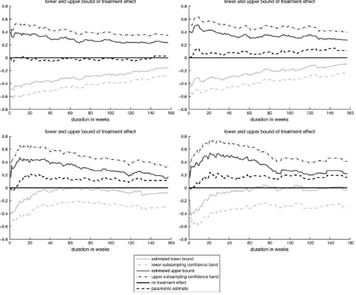
Panels of Figure 3 show worst-case bounds estimates with UPIT and NE as the lower and upper bounds of the unobserved unemployment durations for married males. Top panels show estimates with low preunemployment wages and bottom panels show those with high preunemployment wages. Also, left panels show estimates with the prereform year of 1983 and the postreform year of 1987, and right panels show those with the prereform year of 1983 and the postreform year of 1988. The 95% subsampling pointwise confidence bands, constructed following the procedure in Section 3.2, are also shown along with bounds estimates in Figure 3. The subsample size b is chosen by b ¼n1/2. We found that the results are somewhat sensitive to the choice ofb, but changing the value ofbaround our chosen value would not change our qualitative conclusions. In addition, Figure 3 shows DID estimates with unemployment durations imputed by midpoints between UPIT and NE (i.e., (UPIT þ NE)/2). These estimates are based on untenable imputation methods but are more in line with conventional methods.
For the prereform year of 1983 and the postreform year of 1988, it can be seen that for married males with high pre-unemployment earnings, estimates of lower bounds are more than zero when the unemployment duration is between 15 and 20 months (see the right bottom panel in Fig. 3). In view of the fact that treatment takes place between 12 and 22 months, this provides some evidence on the positive treatment effect. On the other hand, for the same combination of pre- and postreform years, we cannot exclude the possibility of no treatment effect for married males with low preunemployment earnings (see the right top panel in Fig. 3). This does not contradict our con-jecture that the treatment is weak or even not present for this group. This result suggests, in addition, that there is no general worsening of labor market conditions for older employees during this period. This supports the conclusions of Fitzenberger and Wilke (2010), who use the full sample of older unem-ployed persons.
For the pre- and postreform years of 1983 and 1987, we fail to find evidence supporting the positive treatment effect for either income group. Only two representative combinations of pre- and postreform years are shown among six possible combinations of years. Results regarding other combinations of years are in between these two representative combinations and are available on request. For the high preunemployment income group, the lower bound exceeds (at least once) the zero in the relevant time interval (between 12 and 22 months) for all possible combinations of pre- and postreform years. For the low preunemployment group, none of estimates excludes the possibility of no treatment effect. The same conclusion can be drawn with estimates based on imputed unemployment dura-tions by (UPIT þ NE)/2. It can be seen from Figure 3 that estimates are not precise enough to exclude the possibility of no treatment effect in the right bottom panel. Given this, we turn to estimation results with additional restrictions—namely,
^
lðyjxÞand~lðyjxÞin Section 3.
The top panels of Figure 4 show bounds estimates of^lðyjxÞ
and ~lðyjxÞ for married males with low preunemployment
wages, and the bottom panels show those with high pre-unemployment wages. In addition, Table 4 provides bounds estimates and their 95% pointwise confidence intervals fory¼
12, 18, and 24 months. It can be seen that for married males with high preunemployment earnings, the subsampling 95% confidence intervals (in terms of bothl^ðyjxÞ andl~ðyjxÞ) still include zero fory¼18 months. Thus, we have (at best) weak evidence on the positive treatment effect for married males with high preunemployment earnings. In addition, we fail to find any evidence for a treatment effect for married males with low preunemployment earnings even with^lðyjxÞand~lðyjxÞ.
Estimation results of quantile treatment effects tell the same story; thus, they are not reported. Basically, again there is little evidence of the existence of the quantile treatment effect for married males with low preunemployment wages, whereas we can find some evidence of the positive treatment effect at the upper quantiles for those with high preunemployment wages.
We comment on additional estimation results for single males briefly. We find little evidence on the existence of a
treatment effect. For single males with high preunemployment earnings we do not observe a systematic positive treatment effect, because the lower bound exceeds zero only for one possible year combination. Among males, the sample size of the group with a positive treatment effect (based on point estimates of lower and upper bounds) is small compared with all unemployment spells (about 10%; see Table 5). This implies that the treatment effect is small for the full population. Note that a very large share of the unemployment spells in Germany are the result of seasonal unemployment, temporary layoffs, or individuals with short employment spells before unemploy-ment (about 50%). These spells are excluded from our sample because such unemployed persons are not entitled to long-lasting UB transfers. We also did some estimations for this group and did not identify remarkable changes for the treat-ment group.
In addition, we have estimated effects of the reform for different sets of postreform years until 1994 and have found that the results are not substantially different. Estimation
Figure 3. UPIT:l^ðyjx;pt0¼83;pt1¼87Þ; ^uðyjx;pt0¼83;pt1¼87Þ(left) andl^ðyjx;pt0¼83; pt1¼88Þ;u^ðyjx;pt0¼83;pt1¼88Þ(right) for
low (top) and high (bottom) preunemployment wages. Sample restricted to married males.
results are available on request. We make one interesting observation based on these results. When postreform years are extended up to 1994, for the group of married males with high preunemployment incomes, the positive treatment effect per-sists after the end of the treatment. It starts shortly after the beginning of the treatment and it reduces until the end of the treatment. However, after the end of the treatment, the identi-fied effect rises again and it appears to be even stronger than during the treatment period. This could the result of the cumulative effect of the reform. However, it might be the case that something else was going on (e.g., some sort of early retirement).
We end this section by discussing possible sources for estimation bias. One possibility is that if there had been a general worsening in labor market conditions for older employees, this would have led to a right shift of the unem-ployment duration distribution during the postreform period, thereby generating a spurious treatment effect. Although we cannot exclude this possibility, it is unlikely that the estimation results obtained in this section are driven by worsened mac-roeconomic conditions for older employees, given the fact that periods of positive effects match the extension of the maximum length of entitlement for unemployment benefits for the high-income group and no positive effects are identified for the low-income group.
4.2 Inflow to Unemployment
It is also possible to bound changes in the age group com-positions of inflow to unemployment. Details of how to bound these can be found in the Appendix. This allows us to detect whether the layoff behavior of the firms has been changed by the reform. In this subsection we may expect significant changes with respect to the inflow to unemployment just for the
Figure 4. UPIT:l^ðyjxÞ;u^ðyjxÞ(left) and~lðyjxÞ;u~ðyjxÞ(right) for low (top) and high (bottom) preunemployment wages. Sample restricted to
married males.
Table 4. Estimation of treatment effects, sample restricted to married males.
Sample
y¼12 months y¼18 months y¼24 months
lc uc lc uc lc uc
½l^ðyjxÞ;u^ðyjxÞ
Low wage 0.1284 0.2740 0.0430 0.2177 0.0760 0.1770 [–0.32 0.44] [–0.23 0.38] [–0.27 0.34] High wage 0.0106 0.3201 0.0551 0.3033 0.0039 0.2597
[–0.32 0.62] [–0.24 0.60] [–0.30 0.55]
½l~ðyjxÞ;u~ðyjxÞ
Low wage 0.0621 0.1907 0.0430 0.1457 0.0681 0.1156 [–0.25 0.35] [–0.23 0.30] [–0.26 0.27] High wage 0.0106 0.2186 0.0551 0.1904 0.0039 0.1829
[–0.32 0.51] [–0.24 0.47] [–0.30 0.47]
NOTE: Values in brackets are 95% subsampling confidence bands.
subpopulation who increased unemployment duration in response to the reform. For this reason we restrict the analysis to the married males with low or high preunemployment earnings. We use the number of strictly positive UPIT durations as the lower bound for the inflow to unemployment and all NE durations as the upper bound. Intuitively, the lower bound consists only of unemployment durations that are definitely observed, whereas the upper bound comprises all unemploy-ment periods, even those that may be zero.
Table 6 presents the resulting bounds for married males with high or low preunemployment income. For both high and low preunemployment income groups, we do not find any evidence supporting increases in the number of spells in the treatment group. It is difficult to draw a conclusion from this table, but it seems that there is no evidence on changes in the layoff behavior of firms for old workers with high preunemployment earnings.
5. CONCLUSION
This article provides a detailed nonparametric analysis of effects resulting from changes in the German unemployment compensation system using extensive register data. Under mild conditions for our econometric framework we address the important problem of missing information in the data by bounding reform effects according to what the data provide in terms of identification power. As in other articles in the bounds literature, we find that partial identification is a more serious problem than random sampling errors. This suggests that even full population data may not allow precise identification of treatment effects if several administrative registers are not merged with the data accessible to the researcher.
We consider bounds for changes in the inflow and in the duration of unemployment for the treatment group age 44 to 48 years relative to the control group age 36 to 41 years. There is some evidence for the past two decades that the unemployment rate of the treatment group continuously rose relative to the control group (Fig. 5). Using the NE proxy, Lu¨demann, Wilke, and Zhang (2006) do not observe an increase in unemployment duration for the age group 26 to 41 years during recent decades despite a near doubling of the total unemployment rate during this period.
In our analysis we cannot identify that the increase in the unemployment rate of the age group 44 to 48 years is mainly the result of longer search periods of the unemployed in re-sponse to longer entitlement periods for unemployment bene-fits since the mid 1980s. We also do not find evidence for a general worsening of the labor market conditions for the age group 44 to 48 years, because the unemployment durations did not uniformly elongate in all cells of the population. However, there is some evidence for an increase in the length of unemployment duration resulting from the reform. This can be observed for specific subsamples of the data, which amount to
Table 5. Number of spells in the sample, proportion of samples with positive treatment effect
Sample
Prereform years
Postreform years Full sample IABS (males only)
Age 36–41 y 4,445 2,535 Age 44–48 y 3,648 1,982 Sample with positive treatment effect: married
males with high income transfers
Age 36–41 y 533 (12%) 207 (8%) Age 44–48 y 430 (12%) 161 (8%)
Table 6. Changes in inflow to unemployment, sample restricted to married males
Sample
1981 1982 1983
lc uc lc uc lc uc
1987 Low wage 45 117 156 51 134 70 [–53 136] [–181 60] [–156 82] 1987 High wage 15 55 36 53 56 30
[–18 66] [–44 64] [–67 36] 1988 Low wage 61 90 172 24 150 43
[–71 105] [–200 28] [–174 50] 1988 High wage 8 58 29 56 49 33
[–10 70] [–35 67] [–59 40]
NOTE: Values in brackets are 95% bootstrap confidence bands.
Figure 5. Evolution of unemployment rates (left) and difference in unemployment rates of treated and untreated (right). Source: IAB Nuremberg, own calculations.
about 10% of the treated unemployment spells only. In par-ticular, we detect a systematic increase in unemployment spells lasting between 365 and 660 days for married males with high preunemployment income. In several data cells we also identify a general increase in the highest quantiles of the unemployment duration distribution (i.e., after 2 years of unemployment and later). This rise in the length ofverylong-term unemployment (after several years) is likely to make a substantial contribution to the increase in the unemployment rate for this group, but this was not subject to detailed investigation in this article. How-ever, the increase in extreme long-term unemployment may be related to early retirement programs that were conducted dur-ing the period under consideration. It is an interestdur-ing topic for future research. In our estimations, with postreform years up until 1994, we find that the increase in very long-term unem-ployment is much stronger during the years 1991–1994.
Our nonparametric approach is flexible enough to capture different effects over the unemployment spell. Standard dura-tion models such as the propordura-tional hazard model or the accelerated failure time model usually assume a constant or the same sign of the effect over the full unemployment duration. In these models, the estimated increase in unemployment duration for the treatment group after the reform may therefore be driven by the increase in early retirement and not by longer job search periods. The estimation results in the past articles on this topic (except Fitzenberger and Wilke 2010) may be affected because the econometric frameworks applied are not appro-priately specified with this respect. Moreover, we distinguished as far as possible between older unemployed with and without extended entitlement periods and excluded many spells which were not affected by the reform. Finally, there is no evidence on changes in the layoff behavior of firms for old workers with high preunemployment earnings. However, detailed inves-tigation of this has not been covered in this article and will need to be the subject of future research.
The recent reform of the German unemployment compen-sation system led to the merger of UA, IMT, and social bene-fits by the year 2005. The so-called ‘‘new’’ social benebene-fits (Arbeitslosengeld II) is means tested and it is generally at the level of welfare (i.e., it is independent of preunemployment income). In light of the reform in 2006, this suggests that the decrease in the maximum entitlement length for UB will have a stronger effect on individuals with high preunemployment earn-ings than found in this article. This is because the decline in the level of income transfers will be higher than in the old system with UA. However, the size of this group is pretty small compared with the total population of unemployed persons. This may also explain the conflicting results in the past. We therefore con-clude that the effect of the reform on population average search periods will be rather limited. However, as shown by Kyyra¨ and Wilke (2007) for Finland, it will lead to an effective reduction in early retirement for individuals age 55 years and older.
APPENDIX: BOUNDING CHANGES IN THE AGE GROUP COMPOSITION OF THE INFLOW
TO UNEMPLOYMENT
Let N(t, p, x) denote the inflow to unemployment for age group T ¼ t in time period P ¼ p conditional on X ¼ x.
Because we only observe interval data on the duration variable Y,N(t,p,x) is unobserved. However, as before, we can bound N(t,p,x) in the following way. On one hand, forY2(the upper
bound ofY, in our applicationsY2¼NE), we can compute the
inflow toY2, denoted byN2(t,p,x). NoticeN(t,p,x)#N2(t,p, x), becauseY2may contain spells other than unemployment
durations. On the other hand, forY1(the lower bound ofY, in
our applications Y1¼UPIT), we can compute the inflow to
strictly positiveY1, denoted byN1(t,p,x). Notice thatN1(t,p, x)#N(t,p,x), because strictly positiveY1may not contain all
unemployment spells. Also, notice that we consider the inflow only to positive Y1, because the inflow to all Y1 equals the
inflow toY2.
We define the effect of a reform on the age group compo-sition of the inflow to unemployment using the DID frame-work. Specifically, the effect of a reform on the age group composition of the inflow to unemployment (denoted byC(x, pt0,pt1)) is defined as
restrictions over time periods and age groups, Equation (14) implies thatC(x,pt0,pt1) is bounded by an interval with
end-We thank Donald Andrews, Martin Biewen, Hidehiko Ichimura, Charles Manski, Chris Taber, and Gerard van den Berg for helpful discussions; and an associate editor, two anonymous referees, Sarah Bernhard, and Alexander Spermann for useful comments on the article. Comments from the seminar partic-ipants at numerous workshops are also gratefully acknowl-edged. Lee thanks the Economic and Social Research Council and the Leverhulme Trust through the funding of the Centre for Microdata Methods and Practice, and the research program Evidence, Inference and Inquiry. Wilke gratefully acknowl-edges financial support by the German Research Foundation through the research project Microeconometric Modelling of Unemployment Duration under Consideration of the Macro-economic Situation, while he was employed at the Centre for European Economic Research (ZEW Mannheim), Germany.
[Received January 2006. Revised November 2007.]
REFERENCES
Abadie, A. (2005), ‘‘Semiparametric Difference-in-Differences Estimators,’’ The Review of Economic Studies,72, 1–19.
Akritas, M. G. (1986), ‘‘Bootstrapping the Kaplan-Meier Estimator,’’Journal of the American Statistical Association,81, 1032–1038.
Andrews, D. W. K., and Guggenberger, P. (2007), ‘‘Validity of Subsampling and ‘Plug-in Asymptotic’ Inference for Parameters Defined by Moment Inequal-ities,’’ Cowles Foundation Discussion Paper No. 1620, Yale University. Andrews, D. W. K., and Soares, G. (2007), ‘‘Inference for Parameters Defined
by Moment Inequalities Using Generalized Moment Selection,’’ Cowles Foundation Discussion Paper No. 1631, Yale University.
Athey, S., and Imbens, G. W. (2006), ‘‘Identification and Inference in Nonlinear Difference-In-Differences Models,’’Econometrica,74, 431–497.
Bender, S., Haas, A., and Klose, C. (2000), ‘‘The IAB Employment Subsample 1975–1995,’’Schmollers Jahrbuch,120, 649–662.
Bender, S., Hilzendegen, J., Rohwer, G., et al. (1996), ‘‘Die
IAB–Bescha¨ftig-tenstichprobe 1975–1990. Beitra¨ge zur Arbeitsmarkt– und
Ber-ufsforschung.’’ No. 197, Institut fu¨r Arbeitsmarkt- und Berufsforschung der Bundesanstalt fu¨r Arbeit (IAB) Nu¨rnberg.
Beresteanu, A., and Molinari, F. (2008), ‘‘Asymptotic Properties for a Class of Partially Identified Models,’’Econometrica, 76, 763–814.
Biewen, M., and Wilke, R. A. (2005), ‘‘Unemployment Duration and the Length of Entitlement Periods for Unemployment Benefits: Do the IAB Employment Subsample and the German Socio-Economic Panel Yield the Same Results?,’’Allgemeines Statistisches Archiv Vol.,89, 209–236. Blundell, R., Gosling, A., Ichimura, H. et al. (2007), ‘‘Changes in the
Dis-tribution of Male and Female Wages Accounting for Employment Compo-sition Using Bounds,’’Econometrica,75, 323–363.
Bugni, F. A. (2007) ‘‘Bootstrap Inference in Partially Identified Models,’’ unpublished manuscript, Northwestern University, Dept. of Economics. Chernozhukov, V., Hong, H., and Tamer, E. (2007), ‘‘Parameter Set Inference in
a Class of Econometric Models,’’Econometrica,75, 1243–1284.
Fitzenberger, B., and Wilke, R. A. (2010), ‘‘Unemployment Durations in West-Germany Before and After the Reform of the Unemployment Compensation System during the 1980s.’’German Economic Review, 11, forthcoming.
Hall, W. J., and Wellner, J. A. (1980), ‘‘Confidence Bands for a Survival Curve From Censored Data,’’Biometrika,67, 133–143.
Honore´, B. E., and Lleras-Muney, A. (2006), ‘‘Bounds in Competing Risks Models and the War on Cancer,’’Econometrica,74, 1675–1698.
Horowitz, J. L., and Manski, C. F. (2000), ‘‘Nonparametric Analysis of Randomized Experiments With Missing Covariate and Outcome Data,’’ Journal of the American Statistical Association,95, 77–84.
Hujer, R., and Schneider, H. (1995), ‘‘Institutionelle und strukturelle Deter-minanten der Arbeitslosigkeit in Westdeutschland: Eine mikroo¨konomische Analyse mit Paneldaten.’’ in Arbeitslosigkeit und Mo¨glichkeiten ihrer U¨berwindung, Wirtschaftswissenschaftliches Seminar Ottenbeuren, 25, ed. B. Gahlen, H. Hesse, and H. J. Ramser, Tu¨bingen, J.C.B. Mohr, pp. 53– 76.
Hunt, J. (1995), ‘‘The Effect of the Unemployment Compensation on Unem-ployment Duration in Germany,’’Journal of Labor Economics,13, 88–120. Imbens, G. W., and Manski, C. F. (2004), ‘‘Confidence Intervals for Partially
Identified Parameters,’’Econometrica,72, 1845–1857.
Katz, F., and Meyer, B. (1990), ‘‘The Impact of the Potential Duration of Unemployment Benefits on the Duration of Unemployment,’’Journal of Public Economics,41, 45–72.
Kyyra¨, T., and Wilke, R. A. (2007), ‘‘Reduction in the Long-Term Unem-ployment of the Elderly: A Success Story From Finland,’’Journal of the European Economic Association,5, 154–182.
Lechner, M. (1999), ‘‘Nonparametric Bounds on Employment and Income Effects of Continuous Vocational Training in East Germany,’’The Econo-metrics Journal,2, 1–28.
Lu¨demann, E., Wilke, R. A., and Zhang, X. (2006), ‘‘Censored Quantile Regressions and the Length of Unemployment Periods in West Germany,’’ Empirical Economics,31, 1003–1024.
Manski, C. F. (1990), ‘‘Nonparametric Bounds on Treatment Effects,’’ Amer-ican Economic Review Paper and Proceedings,80, 319–323.
——— (1997), ‘‘Monotone Treatment Response,’’Econometrica,65, 1311– 1334.
——— (2003)Partial Identification of Probability Distributions, New York: Springer-Verlag.
Manski, C. F., and Pepper, J. (2000), ‘‘Monotone Instrumental Variables: With Application to the Returns to Schooling,’’Econometrica,68, 997–1010. Manski, C. F., and Tamer, E. (2002), ‘‘Inference on Regressions With Interval
Data on a Regressor or Outcome,’’Econometrica,70, 519–546.
Plaßmann, G. (2002) ‘‘Der Einfluss der Arbeitslosenversicherung auf die Arbeitslosigkeit in Deutschland.’’ Beitra¨ge zur Arbeitsmarkt– und Ber-ufsforschung, 255, Institut fu¨r Arbeitsmarkt- und Berufsforschung der Bundesanstalt fu¨r Arbeit (IAB), Nu¨rnberg.
Romano, J. P., and Shaikh, A. M. (2006a), ‘‘Inference for Identifiable Param-eters in Partially Identified Econometric Models,’’ unpublished working paper, University of Chicago, Dept. of Economics.
——— (2006b), ‘‘Inference for the Identified Set in Partially Identified Econometric Models,’’ unpublished working paper, University of Chicago, Dept. of Economics.
Rosen, A. M. (2008), ‘‘Confidence Sets for Partially Identified Parameters That Satisfy a Finite Number of Moment Inequalities,’’Journal of Econometrics, 146, 107–117.
Schneider, H., and Hujer, R. (1997), ‘‘Wirkungen der Unterstu¨tzungsleistungen auf die Arbeitslosigkeitsdauer in der Bundesrepublik Deutschland: Eine Analyse der Querschnitts- und La¨ngsschnittdimension,’’ in Wirtschafts-und Sozialwissenschaftliche Panel-Studien, Datenstrukturen Wirtschafts-und Analy-severfahren, ed. R. Hujer et al., Sonderhefte zum Allgemeinen Statistischen Archiv, Bd. 30, Go¨ttingen, pp. 71–88.
Van den Berg, G. H. (1990), ‘‘Nonstationarity in Job Search Theory,’’The Review of Economic Studies,57, 255–277.
Wilke, R. A. (2006), ‘‘Semiparametric Estimation of Consumption Based Equivalence Scales: The Case of Germany,’’Journal of Applied Econo-metrics,21, 781–802.