SPATIAL TEMPORAL MODELLING OF PARTICULATE MATTER FOR HEALTH
EFFECTS STUDIES
N. A. S. Hamm
Faculty of Geo-Information Science and Earth Observation (ITC), University of Twente, Enschede, The Netherlands - [email protected]
Commission VIII, WG VIII/2
KEY WORDS:dynamic model, Gaussian process, air quality, particulate mattter, health, low-cost sensors
ABSTRACT:
Epidemiological studies of the health effects of air pollution require estimation of individual exposure. It is not possible to obtain measurements at all relevant locations so it is necessary to predict at these space-time locations, either on the basis of dispersion from emission sources or by interpolating observations. This study used data obtained from a low-cost sensor network of 32 air quality monitoring stations in the Dutch city of Eindhoven, which make up the ILM (innovative air (quality) measurement system). These stations currently provide PM10 and PM2.5 (particulate matter less than 10 and 2.5 m in diameter), aggregated to hourly means. The data provide an unprecedented level of spatial and temporal detail for a city of this size. Despite these benefits the time series of measurements is characterized by missing values and noisy values. In this paper a space-time analysis is presented that is based on a dynamic model for the temporal component and a Gaussian process geostatistical for the spatial component. Spatial-temporal variability was dominated by the temporal component, although the spatial variability was also substantial. The model delivered
accurate predictions for both isolated missing values and 24-hour periods of missing values (RMSE = 1.4µg m−3
and 1.8µg m−3
respectively). Outliers could be detected by comparison to the 95% prediction interval. The model shows promise for predicting missing values, outlier detection and for mapping to support health impact studies.
1. INTRODUCTION
Epidemiological studies of the health effects of air pollution re-quire estimation of individual exposure. Such studies typically aim to identify the outdoor air pollution concentration at subjects residence, school or place of work. This is then used to quan-tify exposure. Idenquan-tifying the air pollution concentration at rele-vant locations, for given points or periods in time, is challenging because it is not possible to obtain measurements at all relevant locations. It is therefore necessary to predict at these space-time locations, either on the basis of dispersion from emission sources or by interpolating observations. This study uses data obtained from a low-cost sensor network of 32 air quality monitoring sta-tions in the Dutch city of Eindhoven, which make up the ILM (in-novatief luchtmeetsysteem/innovative air (quality) measurement system) (Hamm et al., 2016). These stations currently provide PM10 and PM2.5 (particulate matter less than 10 and 2.5 m in diameter), aggregated to hourly means. The data provide an un-precedented level of spatial and temporal detail for a city of this size.
Analysis of space-time data has received a lot of attention in re-cent years. The ILM data can be considered discrete in time (they refer to specific one-hour periods) but continuous in space. The approach taken in this paper follows Gelfand et al. (2005) and Finley et al. (2012) and treats the data as arising from time series of spatial processes, where a dynamic model describes the temporal evolution of the data. This is described further in Sec-tion 3.
Various data quality challenges arise when analysing these data. First, for each sensor there may be missing observations ranging from isolated values to a series of several weeks (e.g., if an instru-ment is removed for maintenance). Second, the data are typically noisy by comparison to conventional observations and this may lead to unreliable observations. It is necessary to identify these
unreliable observation and remove them or correct them. Third, it is necessary to identify the requirements for the epidemiologi-cal study in terms of the spatial and temporal resolution and the precision of the interpolated values. This study addressed the first two problems.
2. STUDY AREA AND DATA
The study site is Eindhoven, a city in the south of the Netherlands
(municipal population 220,000, municipal area 90 km2
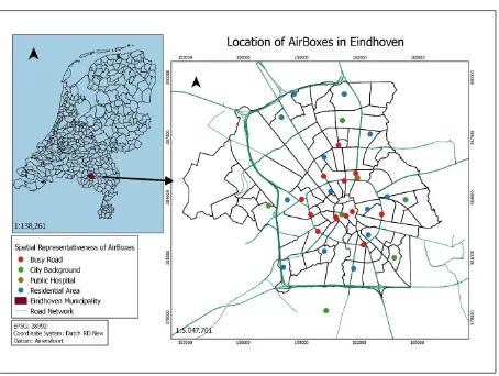
). Eind-hoven is home to the AiREAS initative, which is a cooperative venture that unites industry, local government, universities, small business and civic organizations towards the goal of a healthy and sustainable city (Close, 2016). As part of this initiative an in-novative outdoor low-cost was installed in 2012, comprised of 32 Airboxes (Figure 1). Each Airbox contains a control and telecom-munication unit as well as low-cost sensors that measure the con-centration of different air pollutants. In this paper, the focus is
on particulate matter (PM), particularly PM10 (PM< 10µm in
diameter), which is measured at every Airbox using an optical system. The locations of the sensors were chosen to reflect (i) sources of pollution (e.g., roads, junctions) (ii) places where peo-ple live and spend their time (iii) background locations. All sen-sors were calibrated against a beta attenuation monitoring (BAM) instrument prior to installation in autumn/winter 2013 (Hamm et al., 2016). The BAM instrument is part of the official Dutch air quality monitoring network, maintained by RIVM (National In-stitute for Public Health and the Environment). Background in-formation to the ILM is given by Hamm et al. (2016). The data used for this study were hourly data for a 2-week period from 1-14 October 201-14 where a complete set of hourly data for PM1, PM2.5 and PM10 were available. This led to 336 observations
(24 hours×14 days) at 32 locations.
In addition to the air quality data, hourly meteorological data
The International Archives of the Photogrammetry, Remote Sensing and Spatial Information Sciences, Volume XLI-B8 2016 XXIII ISPRS Congress, 12–19 July 2016, Prague, Czech Republic
This contribution has been peer-reviewed.
Figure 3 Spatial representativeness of ILM network in Eindhoven
Figure 1. Location of airboxes in Eindhoven
were available for a single station in Eindhoven, maintained by the Royal Netherlands Meteorological Institute (KNMI).
3. METHODS
Consider thatyt(s)is the observation (e.g., PM10) at location,s,
and time,t. The model is built up firstly through ameasurement
equation:
yt(s) =xt(s)′βt+ut(s) +εt (1)
wherex
t(s)is a vector ofpcovariates, which may vary in space,
andβtis ap×1vector of regression coefficients which are
con-stant in space for a given time. The termut(s)is a space-time
varying intercept whilstεt
ind
∼N(0, τ2
t) is the spatially and
tem-porally uncorrelated error. Nexttransition equationsmodel the
time varying regression coefficients,βt:
βt=βt−1+ηt, ηt
iid
∼N(0,Ση) (2)
and the space-time varying intercept,ut(s):
ut(s) =ut−1(s) +wt(s) (3)
wherewt(s) ∼ GP(0, Ct(·,θt))fort = 1, . . . , nt andGP
refers to a spatialGaussian ProcesswhereCt(·,θt))is the
spa-tial covariance function. For a covariance function with a single
decay parameter, θt = (σ
2
t, φt), whereφ is the spatial decay
parameter, often referred to as the range. Considering the
com-monly used exponential correlation function,Ct(s1,s2;θt)) =
σ2
tρ(s1,s2;φt) =σ
2
texp(−φt||s1−s2||), whereh=||s1−s2||
is the Euclidean lag distance betweens1ands2.
Implementation followed the approach set out in Finley et al. (2012). The model parameters were estimated in a Bayesian framework using Markov Chain Monte Carlo (MCMC) simula-tion. Non-informative priors were used for all paramters: Normal
distributions for theβ’s, uniform distributes for theφ’s, inverse
Gamma distributions for theτ2
’s andσ2
’s and inverse Wishart
forΣη. The MCMC was implemented usingspBayes(Finley
et al., 2007) in the R software (R Core Team, 2016) for a chain of length 20,000 with the first 15,000 being discarded as burn-in. Chain trace plots were examined for convergence and inference was conducted using the remaining 5000 samples.
Three experiments were conducted.
1. 500 measurements were removed at random. This experi-ment recreates the sitution of isolated missing observations
(∼5% of all observations) that need to be filled-in in order
to have a complete time series.
2. Three complete days of measurements were removed (day 8 for sensors 9, 12 and 18). This experiment recreates the situation where sensors are removed for extended periods.
3. The results were queried for outlying observations, which were then cleaned from the dataset.
4. RESULTS
For this research, space varying covariates were not available. However, exploratory analysis of the temporal variability in PM10 against the meteorological variables did not reveal any clear cor-relation. There was also no clear association between the type of monitoring station (e.g., background, busy street, residential street) and PM10 concentration. Subsequent analysis proceeded
without covariates in Equation 1, hencep= 1andxt= 1.
4.1 Experiment 1
Figure 2 shows the time-series of the temporally varying mean,
βt. This can be interpreted as the dynamic time signal in the
data. The time specific estimates of the variance parameters (τ2
t,
σ2
t andφ) are shown in Figure 3. There was clear evidence of
spatial structure at most points in time, with a typical median
value ofσ2
t/(τ
2
t +σ
2
t) = 0.6. Large values ofτ
2
t or low
val-ues ofφwere typically associated with outliers (see Section 4.3).
The temporal component was larger than the spatial component
withΣη= 6.13(5.24,7.19)(values in parentheses give the 95%
credible interval) andσ2
t as illustrated in Figure 3.
●● ● ● ● ● ●● ●
● ● ●
●
● ●●●
● ● ● ● ●
●
● ● ● ● ● ● ●
●
● ● ● ●●●●
●● ● ● ● ● ● ● ● ● ● ● ● ● ● ● ●
●
●
●
●
●
● ● ●●●●●●
●● ●●● ● ●●●
● ●● ● ●● ●● ●●●●
●● ● ●●● ● ● ● ● ● ●● ● ● ● ● ● ● ●● ● ● ● ●● ● ●● ● ● ●●● ● ●● ● ● ● ●● ● ●● ● ● ● ● ● ● ● ●● ●● ● ●● ●● ● ● ● ● ● ● ● ● ●
● ●●●●●●
●● ●● ●●●●
● ● ● ● ● ●●
●
●
● ● ● ● ● ●●● ●● ●● ● ● ● ●● ● ●● ● ●● ●●●
● ●●●
● ●●●●
●●● ● ● ●●
● ● ●●●●●
●●●●●●●●● ●●●●
●●● ●●●●●●●●●●●●●
●●●●●●● ● ● ●●●
● ●
●● ●● ●● ● ● ●●
● ● ● ● ● ● ● ● ● ● ● ● ●
● ● ● ● ●
● ● ● ● ● ● ●●●
● ● ●
● ● ● ● ●
●
●
● ● ● ●
● ●
●
●● ● ●● ● ●
0 50 100 150 200 250 300
0
10
20
30
40
hours
beta
●● ● ● ● ● ●● ●
● ● ●
●
● ●●●
● ● ● ● ●
●
● ● ● ● ● ● ●
●
● ● ● ●●●●
●● ● ● ● ● ● ● ● ● ● ● ● ● ● ● ●
●
●
●
●
●
● ● ●●●●●●
●● ●●● ● ●●●
● ●● ● ●● ●● ●●●●
●● ● ●●● ● ● ● ● ● ●● ● ● ● ● ● ● ●● ● ● ● ●● ● ●● ● ● ●●● ● ●● ● ● ● ●● ● ●● ● ● ● ● ● ● ● ●● ●● ● ●● ●● ● ● ● ● ● ● ● ● ●
● ●●●●●●
●● ●● ●●●●
● ● ● ● ● ●●
●
●
● ● ● ● ● ●●● ●● ●● ● ● ● ●● ● ●● ● ●● ●●●
● ●●●
● ●●●●
●●● ● ● ●●
● ● ●●●●●
●●●●●●●●● ●●●●
●●● ●●●●●●●●●●●●●
●●●●●●● ● ● ●●●
● ●
●● ●● ●● ● ● ●●
● ● ● ● ● ● ● ● ● ● ● ● ●
● ● ● ● ●
● ● ● ● ● ● ●●●
● ● ●
● ● ● ● ●
●
●
● ● ● ●
● ●
●
●● ● ●● ● ●
Figure 2. Variation inβtover time (median (red dot) and 95%
credible interval).
An example time-series plot of the predicted values is shown in
Figure 4 for Airbox 16. Note that βt is the same at all
loca-tions (see Equation 2, whereasut(s)differs between locations
(see Equation 3) and the predicted value is the sum of these two components. The isolated missing values were not observable on the prediction plots; however, the measured values were
consis-tent with the 95% credible interval and the RMSE was 1.4µg
m−3
across the 500 missing values.
4.2 Experiment 2
Figure 5 shows prediction at Airboxes 9. For Airbox 9 the mea-surements were removed on Day 8 for the modelling stage. The median prediction closely matched the observed values (RMSE=1.8
µg m−3
) although the credible interval was clearly wider than at
The International Archives of the Photogrammetry, Remote Sensing and Spatial Information Sciences, Volume XLI-B8 2016 XXIII ISPRS Congress, 12–19 July 2016, Prague, Czech Republic
This contribution has been peer-reviewed.
●
hours
sigma.sq
●
hours
tau.sq
●●●●●
hours
eff
. r
ange (km)
●
Figure 3. Variation inσ2
t (top),τ
2
t (middle), and3/φ(effective
range) (bottom) over time (median and 95% credible interval).
0 50 100 150 200 250 300
hours
PM10
●●●●
Figure 4. Predictions of PM10 at Airbox 16. Included are the
95% prediction interval (grey region), medianβt(red dots),
me-dianut(s9)(green dots), median prediction (i.e.,βt+ut(s9))
(blue dots), observed value (open black circles).
other points in time or for Airbox 16 (Figure 4), where observa-tions were not removed. This is as expected, since no measure-ments were available to support prediction.
4.3 Experiment 3
As well as prediciting missing values, this study also yielded re-sults that are useful for identifying outliers. Figure 4 shows that there are some isolated observations that lie outside the 95% cred-ible interval. Following the approach of Zhang et al. (2012) these may be considered outliers. Further, the very wide credible
in-0 50 100 150 200 250 300
hours
PM10
●●
Figure 5. Predictions of PM10 at Airbox 9. Vertical lines indicate Day 8 where the observations were predicted but not included in the modelling stage. Other details are as in Figure 4.
terval at hour 62 (Figure5) arose because a single extreme value
at Airbox 6 (PM10 = 83µg m−3
) leading to a large estimated
value forτ2
62. Removing these values and re-doing the modelling
removes these outliers and very large value ofτ2
62.
5. DISCUSSION AND CONCLUSIONS
The lack of correlation with meteorological variables should not be taken as a general result. It may simply be that there was no correlation within this time period. This should be re-evaluated when implementing the model for other time periods. Future ef-forts should consider space-varying covariates as well as time-varying covariates that do not have a spatial component (e.g., via Equation 2. Space-time varying covariates have recently become available (Dash, 2016) and will be evaluated in future implemen-tations. Dash (2016) also used a dispersion model output as a covariate, an approach which has been successful at coarser res-olutions (Akita et al., 2014; Hamm et al., 2015).
The proposed model yielded accurate predictions of isolated miss-ing values (Experiment 1) as well smiss-ingle days of missmiss-ing values (Experiment 3). Although further evaluation is required, this ap-proach shows promise as a method that could be used to fill in missing values and provide a complete time series to users. A fur-ther step is to make predictions at unsampled locations, leading to the production of space-time maps, as proposed by (Gelfand et al., 2005) and (Finley et al., 2012). When such maps are to be used in the context of environmental epidemiological studies, further investigation would be required to identify the required space-time resolution, as well as the required accuracy.
Finally, outliers were identified in an interactive fashion by com-paring the observed values to the predictions and the associated 95% credible interval. Isolated outliers were identified and re-moved from the dataset. These could then be replaced by the pre-dicted values. Extreme outliers could influence inference (e.g., hour 62 at Airbox 6), so it was necessary to re-run the analysis after removing these outliers. This approach presented in this pa-per requires further evaluation but shows promise as method for interactive removal of outliers. A future step would be to use it for automated outlier detection.
This paper has addressed the initial stages of space-time mod-elling of particulate matter for a novel low-cost sensor network that delivers observations at a fine spatial and temporal resolution. Future work needs to identify the spatial and temporal resolution
The International Archives of the Photogrammetry, Remote Sensing and Spatial Information Sciences, Volume XLI-B8 2016 XXIII ISPRS Congress, 12–19 July 2016, Prague, Czech Republic
This contribution has been peer-reviewed.
that is achievable for predictive mapping. This is important be-cause it will influence the health questions that can be addressed.
References
Akita, Y., Baldasano, J. M., Beelen, R., Cirach, M., de Hoogh, K., Hoek, G., Nieuwenhuijsen, M., Serre, M. L. and de Nazelle, A., 2014. Large scale air pollution estimation method combin-ing land use regression and chemical transport modelcombin-ing in a
geostatistical framework. Environmental Science &
Technol-ogy48(8), pp. 4452–4459.
Close, J.-P. (ed.), 2016. AiREAS: Sustainocracy for a Healthy
City. Springer. DOI: 10.1007/978-3-319-26940-5, Dordrecht.
Dash, I., 2016. Space-time observations for city level air quality modelling and mapping. Master’s thesis, University of Twente, The Netherlands.
Finley, A., Banerjee, S. and Carlin, B., 2007. spBayes: An
R package for univariate and multivariate hierarchical
point-referenced spatial models. Journal of Statistical Software
19(1), pp. doi: 10.18637/jss.v019.i04.
Finley, A. O., Banerjee, S. and Gelfand, A. E., 2012. Bayesian dynamic modeling for large space-time datasets using
Gaus-sian predictive processes. Journal of Geographical Systems
14(1), pp. 29–47.
Gelfand, A. E., Banerjee, S. and Gamerman, D., 2005. Spatial process modelling for univariate and multivariate dynamic
spa-tial data.Environmetrics16(5), pp. 465–479.
Hamm, N. A. S., Finley, A. O., Schaap, M. and Stein, A., 2015. A spatially varying coefficient model for mapping air quality
at the European scale.Atmospheric Environment102, pp. 393–
405.
Hamm, N. A. S., van Lochem, M., Hoek, G., Otjes, R., van der Sterren, S. and Verhoeven, H., 2016. The invisible made
vis-ible: Science and technology. In: J.-P. Close (ed.),AiREAS:
Sustainocracy for a Healthy City: The Invisible made Visible Phase 1, Springer, Dordrecht, pp. 51–77.
R Core Team, 2016. R: A Language and Environment for Sta-tistical Computing. R Foundation for StaSta-tistical Computing, Vienna, Austria.
Zhang, Y., Hamm, N. A. S., Meratnia, N., Stein, A., van de Voort, M. and Havinga, P. J. M., 2012. Statistics-based outlier
de-tection for wireless sensor networks. International Journal of
Geographical Information Science26(8), pp. 1373–1392.
The International Archives of the Photogrammetry, Remote Sensing and Spatial Information Sciences, Volume XLI-B8 2016 XXIII ISPRS Congress, 12–19 July 2016, Prague, Czech Republic
This contribution has been peer-reviewed.