BIODIVERSITY MAPPING VIA NATURA 2000 CONSERVATION STATUS AND EBV
ASSESSMENT USING AIRBORNE LASER SCANNING IN ALKALI GRASSLANDS
A. Zlinszky a, B. Deák b,c, A. Kania d, A. Schroiff e, N. Pfeifer d, * a
Centre for Ecological Research, Hungarian Academy of Sciences, 8237 Tihany, Hungary – [email protected] b
MTA-DE Biodiversity and Ecosystem Services Research Group, 4032 Debrecen, Hungary – [email protected] c Technische Universität Bergakademie Freiberg, Interdisciplinary Ecological Centre, D-09596 Freiberg, Germany
d
Department of Geodesy and Geoinformation, Technische Universität Wien, 1040 Vienna, Austria – [email protected]
e
YggdrasilDiemer, 10965 Berlin, Germany – [email protected]
ThS 10 – Spatial ecology and ecosystem services mapping using Essential Biodiversity Variables
KEY WORDS: LIDAR, Essential Biodiversity Variables, Natura 2000, Conservation status, Biodiversity assessment
ABSTRACT:
Biodiversity is an ecological concept, which essentially involves a complex sum of several indicators. One widely accepted such set of indicators is prescribed for habitat conservation status assessment within Natura 2000, a continental-scale conservation programme of the European Union. Essential Biodiversity Variables are a set of indicators designed to be relevant for biodiversity and suitable for global-scale operational monitoring. Here we revisit a study of Natura 2000 conservation status mapping via airbone LIDAR that develops individual remote sensing-derived proxies for every parameter required by the Natura 2000 manual, from the perspective of developing regional-scale Essential Biodiversity Variables. Based on leaf-on and leaf-off point clouds (10 pt/m2) collected in an alkali grassland area, a set of data products were calculated at 0.5 ×0.5 m resolution. These represent various aspects of radiometric and geometric texture. A Random Forest machine learning classifier was developed to create fuzzy vegetation maps of classes of interest based on these data products. In the next step, either classification results or LIDAR data products were selected as proxies for individual Natura 2000 conservation status variables, and fine-tuned based on field references. These proxies showed adequate performance and were summarized to deliver Natura 2000 conservation status with 80% overall accuracy compared to field references. This study draws attention to the potential of LIDAR for regional-scale Essential Biodiversity variables, and also holds implications for global-scale mapping. These are (i) the use of sensor data products together with habitat-level classification, (ii) the utility of seasonal data, including for non-seasonal variables such as grassland canopy structure, and (iii) the potential of fuzzy mapping-derived class probabilities as proxies for species presence and absence.
* Corresponding author
1. INTRODUCTION
1.1 Natura 2000 and Essential Biodiversity Variables
The ongoing biodiversity crisis has fuelled increasing efforts to quantify and map biodiversity, both for monitoring purposes and for a deeper scientific understanding. Biodiversity, defined as the variability of all living organisms, is a complex phenomenon with many different levels, therefore difficult to quantify with a single indicator. The Natura 2000 network of the European Union, which was established by the Habitats Directive (European Commission, 1992) is monitored by assessing the conservation status of each site every six years. Conservation status is based on a system health approach and the indicator itself is defined as a weighted sum of several variables, each related to different aspects of the habitat. The directive requires that characteristic species, structure of the habitat, human influence and future prospects be assessed through individual proxies, and combined to output a final conservation status on a categorical scale of A (favourable), B, (unfavourable –inadequate) of C (unfavourable-bad).
Essential Biodiversity Variables (EBV-s) take a less complex approach, they are "a measurement required for study, reporting and management of biodiversity change" (Pereira et al., 2013), keeping in mind that “any attempt to define a set of variables for tracking biodiversity change should indeed ensure that
information on all components and dimensions of biodiversity are being captured” (Pettorelli et al., 2016). In this sense, they represent spatially explicit and scalable proxies of individual biophysical variables that are relevant to biodiversity by influencing it in some way or being closely linked to an important aspect of it. The idea of EBV-s was raised with global-scale satellite remote sensing-based monitoring in mind and global data coverage is regarded as a requirement towards candidate EBV-s (Pettorelli et al., 2016), but biodiversity monitoring at a finer scale is also in demand, both from the side of decision support and scientific research. Identifying measurable variables that "balance specificity and generality, enabling valid aggregation of data from multiple monitoring programs, while allowing for flexibility in the species or taxonomic groups addressed by these programs" (Pereira et al., 2013) is just as relevant at this scale as it is globally, since conservation action takes place at national or regional level. At regional scale and national to continental coverage, not only satellite-based sensor products may be considered but also airborne sensors. Airborne LIDAR has been identified to hold especially high potential for biodiversity monitoring (Simonson et al., 2014; Zlinszky et al., 2015b) due to its ability to capture three-dimensional spatial structure in high resolution together with radiometric properties in a spectral band relevant for ecophysiology. Studies have proven that LIDAR can be used even on its own for detailed phytosociological classification or The International Archives of the Photogrammetry, Remote Sensing and Spatial Information Sciences, Volume XLI-B8, 2016
vegetation health studies, both in forests (Maltamo et al., 2014) and in herbaceous vegetation (Zlinszky et al., 2014, 2012). Meanwhile, data coverage continues to increase both through ongoing national survey projects and dedicated campaigns at individual sites serving a wide variety of purposes. This means that LIDAR will play an important role in regional-scale biodiversity monitoring (Zlinszky et al., 2015b).
1.2 Objectives
In this study we revisit a dataset collected originally for the purpose of developing LIDAR as a tool for Natura 2000 monitoring (Zlinszky et al., 2015a) from the perspective of identifying potential EBV-s. The original study aimed to create proxies for all variables required by the national Natura 2000 monitoring guidelines, using only LIDAR data and field references, and based on these, to create a high-resolution complete Natura 2000 conservation status assessment for the study area. Here we investigate the processing steps and results in order to identify LIDAR-based Essential Biodiversity Variables that could potentially support regional-scale biodiversity monitoring also beyond the framework of Natura 2000.
2. DATA AND METHODS
2.1 Study Site and Input Data
The methodology used for data collection and processing is
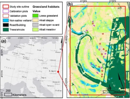
described in detail in (Zlinszky et al., 2015a) and briefly summarized here. The study area is Ágota-puszta (Fig. 1), a Natura 2000 site within the Hortobágy Special Area of Conservation. The local vegetation is dominated by "1530 Pannonic Salt Steppes and Salt Marshes" Natura 2000 habitat type (European Commission DG Environment, 2007), which represents a mosaic of arid, semi-arid and wet, but always salt-tolerant grass- and forb-dominated vegetation. The micro-topography has low relief but high variability, and creates locally very diverse water and soil conditions that result in a tightly-knit pattern of various grassland associations (Deák et al., 2014; Molnár and Máté, 2014). The site is used for extensive cattle grazing.
Field references were collected at two individual levels (Zlinszky et al., 2015a): for the individual classifications and for the final Natura 2000 conservation status. Both datasets were split with half of the polygons used for calibration and half retained for accuracy evaluation. At the first level, 364 separate polygons of approximately 25 m2 each were located with sub-meter accuracy using Differential GPS, noting vegetation class and also biodiversity-relevant features such as trampling, grazing, occurrence of weeds). At the second level, 20 sample plots of 50 m × 50 m were selected in a layout to cover the full range of grassland associations present in the area and their conservation status available at the site, and complete Natura 2000 conservation status assessment surveys were carried out within each.
The Hungarian Natura 2000 Conservation Status assessment scheme for grasslands requests 13 individual variables to be
Figure 1. Location of the study site in Central Europe (a), overview of the study site including land cover, main alkali grassland classes and Natura 2000 conservation status reference plots. Reproduced with permission from (Zlinszky
2015a)
surveyed, each with a pre-defined protocol (Zlinszky et al., 2015a). The plot receives a positive or negative score depending on the status of the plot with respect to each variable (favourable or unfavourable), with the magnitude of the score representing the weighting assigned to the variable. For example, if no shrub encroachment is observed, +5 points are scored, if encroachment is present, the score is -1, if an invasive alien shrub species is present, it is -10. The final status is defined by summing the positive and negative scores separately. If the positive score reaches 50 and the negative is not less than -10, the conservation status is favourable (A). If the negative score is less than -20, the status is unfavourable-bad (C), in all other cases, it is unfavourable-inadequate (B). The 13 variables prescribed by the assessment scheme are naturalness, species density, inner patchiness, vertical structure, species pool, litter accumulation, soil erosion, shrub encroachment, weed growth, human disturbance, future threats, animal traces and landscape context (see Zlinszky 2015a for full details). Each of these has a pre-defined methodology for mapping in the field, which we followed during ground truthing and attempted to copy during LIDAR data processing.
LIDAR data was collected using a Riegl LMSQ680i full-waveform scanner, operating at 1550 nm wavelength. The flying height of ca. 620 m above ground level resulted in 10 pt/m2 nominal stripwise echo density and a footprint size of approximately 20 cm diameter. The full study area of 24 km2 was scanned twice, once before the growth season in March 2013 and once at the peak of the growing season in June 2013 when the grass and herb dominated vegetation is the most developed.
2.2 Data Processing and Accuracy Analysis
The point clouds were radiometrically corrected based on field spectroscopy measurements (Lehner and Briese, 2010). A set of output raster products was calculated from the point clouds using OPALS software (Pfeifer et al., 2014), always with 0.5 m × 0.5 m raster cell size. These products include a digital terrain model (DTM) based on iterative robust interpolation of the leaf-off point cloud (Pfeifer et al., 2001), a canopy height model of the maximum relative height above the DTM in each raster cell, mean and variance of point reflectances, mean and maximum point echo width (EW) and EW variance, and finally a set of surface texture measures (point height variance, sigma, and openness) within the raster cells using two different kernel sizes (3 × 3 and 5 × 5 pixels). For each of these data products, the difference between the leaf-on and leaf-off values were also calculated as separate raster layers. All in all this resulted in a multi-band pseudo-image of 70 LIDAR data products, which was the basis of vegetation classification and feature detection. For this, we developed and used the Vegetation Classification Studio (VCS) software tool (Zlinszky and Kania, 2016) to train a random forest machine learning classifier (Breiman, 2001; Pedregosa et al., 2011) that supports fuzzy class prediction output, visualization and accuracy evaluation. In fuzzy classification, each pixel is assigned not only a single class but a vector representing the probabilities of the pixel belonging to each of the individual classes. VCS allows classification schemes created from the same set of reference data with a hierarchical class structure. High computation and rendering
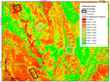
Figure 2: Fine-tuning threshold value for the conservation status variable "species density", represented by variance of leaf-on reflectance. According to this map the correct threshold value would be 0.002. Reproduced with permission
from Zlinszky et al.(2015a)
performance is achieved by decoupling classifier training and evaluation which is only carried out on the subset of the data reserved for training and validation from rendering and visualization with adaptive resolution to support fast viewing of the prediction on the full dataset (Kania and Zlinszky, 2014). For this study, five different classification products were calculated in a hierarchical categorization: 4 land cover classes, 8 main alkali habitat classes, 15 grassland vegetation associations, 5 classes representing disturbance, 5 classes relevant for shrub encroachment in each case based on the first level of ground truthing.
In the next step, LIDAR-based proxies for each of the variables required by the Natura 2000 assessment scheme had to be identified. These were either probabilities of individual categories based on the fuzzy classification products listed above ( within this section 2.2), or direct LIDAR sensor product datasets (listed in section 2.1). Since the scheme requires surveying not on a numerical scale but on a categorical scale of 2-4 steps, calibration could also only be carried out with this level of detail. The thresholds separating favourable or unfavourable status for the individual variables were pre-selected to follow the rules laid down in the Natura 2000 field
assessment scheme, and the exact values were fine-tuned using the respective parameter values in the 10 calibration plots (Fig. 2).
Wherever possible, we aimed to directly use the output of the relevant classification (such as for weeds or shrubs), and find a LIDAR sensor product where relevance had a plausible explanation (such as normalized height for vertical structure). For parameters where all calibration plots had the same value, the fine-tuning step had to be omitted.
Accuracy was evaluated separately for each parameter. Since the Natura 2000 CS field evaluation plots held ca. 10000 raster pixels each, but were observed in the field to have homogeneous values within their area for each individual CS parameter, the ratio of pixels assigned to the correct status by the LIDAR classifier was a strong indicator of accuracy as long as differences in status were present among the validation plots. This could be investigated through the 10 different validation plots which held different conservation status scores for different variables. The summed conservation status scores based on the LIDAR data were also compared with the respective field-observed scores. The final status assigned to each plot by summing all variables and applying the pre-defined
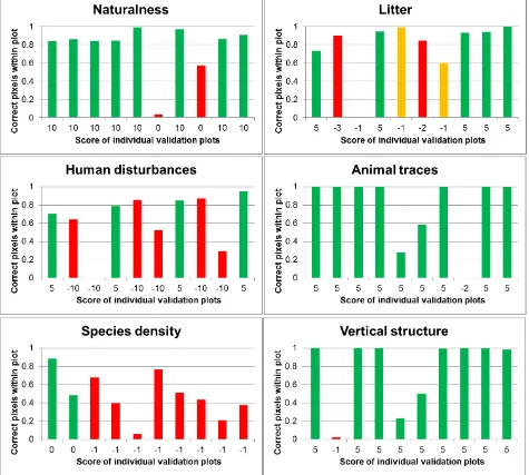
Figure 3: Ratio of correctly categorized validation plot pixels based on LIDAR data for individual conservation status parameters. Red and orange columns represent unfavourable status for the respective indicator, green columns stand for favourable status
thresholds from the Natura 2000 field assessment manual was also compared between the field-based and LIDAR-based results.
3. RESULTS
The individual classification products all showed good agreement with their respective ground truths, with Cohen's Kappa values ranging from 0.58 (for grassland associations) to 0.83 (land cover) (Zlinszky et al., 2015a). However, evaluation was not always possible due to the distribution of the ground truth values (Zlinszky et al., 2015a). For the individual CS-relevant parameters, one of the most important findings was that different threshold values separating favourable or unfavourable status apply for different grassland association types within the main category. Therefore, tall-grass associations (alkali meadows) were separated from short-grass associations (alkali swards and open steppes) based on the main alkali habitat class map. After this step, the following proxies were identified: From the directly derived sensor data products, the difference between leaf-on and leaf-off mean point reflectance within the raster cells proved to be a reliable representation of the grazing regime, successfully identifying over- and undergrazed patches. This means it was a relevant proxy for “naturalness”, “litter accumulation”, “animal traces” and partly for “human disturbances”, which are four different variables requested by the Natura 2000 monitoring scheme. Different thresholds were applied to this LIDAR product for representing these different variables; accordingly the accuracy also varied (Fig. 3). 83% of the validation pixels was correctly labelled for “naturalness”, 2 out of 10 plots had unfavourable naturalness, one of these was correctly identified. 82% of the full validation area was correct for “animal traces”, but the single unfavourable case was not well recognized. 79% of the pixels were correct for litter accumulation, and both favourable and unfavourable cases were mostly well identified. For disturbance, which also included another LIDAR product, 64% of the pixels were correctly labelled (see below).
Based on the spectral variation hypothesis (Palmer et al., 2002), “species density” was represented with the variance of leaf-on point reflectance within a neighbourhood. Different kernel sizes were applied to the short and long-grass habitats to follow their characteristic patch scales, but the threshold was the same. However, only 47% of the pixels were assigned the correct status with this approach, but there seems to be no bias towards the favourable or unfavourable cases.
The difference in leaf-on and leaf-off normalized height was used as a representation of the conservation status variable “vertical structure”. The field manual defines this parameter based on the coverage of typical overstory, medium level and understory grass and herb species and not physical heights. This explains why vertical strucutre did not perform well, completely missing the single unfavourable case.
For “disturbances”, the value of the seasonal difference in reflectance (a proxy of overgrazing) was combined through a logical OR operation with the probability of the class "vehicle track" from the disturbance classification. The resulting accuracy was 64%, but for this particular variable, not all reference plots could be considered homogeneous, as e.g. a field road would only affect part of the reference plot.
For the other variables, accuracy could not be assessed with this method, since the validation plots did not contain all possible cases. Using the products of the fuzzy classification, the conservation status variable “species pool” was found to be well represented by the summed probability of vegetation associations belonging to the grassland habitat in focus. It was class from the disturbance classification, assigning a fix threshold to separate favourable and unfavourable status. However, indicator accuracy could not be tested as no validation plots had weeds; therefore, it corresponds to the accuracy of the relevant class (69% F1-score, (Zlinszky et al., 2015a)).
Similarly, “shrub encroachment” was represented by the dedicated classification product which separately included invasive shrubs as a class. However, here instead of probability, the hard-boundary result was used, complemented by a morphological operation to identify dense stands which represent the worst status according to the field Natura 2000 evaluation scheme. Accuracy in this case also corresponds to the classification accuracy, which is 70% (mean F1-score of native and invasive shrub classes, (Zlinszky et al., 2015a)). For 4 out of the 13 parameters required by the assessment scheme, all reference plots (even the calibration plots) had the same status, therefore indicator variables were assigned but not quantitatively evaluated. For "future threats" the most important threat to this protected area observed in the field was lowering of the water table. DTM height represents distance to the groundwater table at this scale and was therefore expected to be a good proxy of this threat. All field references were assessed to be negatively affected by this risk, therefore the threshold was set at a height below the lowest calibration plot. Based on terrain model height accuracy, this proxy is expected to be valid in 95% of the cases, but this could not be directly evaluated. “Patchiness of vegetation” is also a CS parameter, however, it is less relevant to this habitat type which is always highly patchy. Therefore, all areas within the land cover class "alkali grassland" were assigned high patchiness. The class “alkali grasslands” of the land cover classification has 95% accuracy (F1-score). “Soil erosion” was also represented by the same indicator, as soil erosion has a favourable effect on this habitat type.
Finally, “landscape context”, which represents the neighbouring habitats, and the distance to the nearest similar habitat, was evaluated using pixel counts within a kernel: if alkali grasslands dominated the local neighbourhood and occurred within a 100 m distance, then this parameter had favourable status.
The individual uncertainties and errors of these proxy variables are partly averaged out by the aggregation process that sums the respective scores of the parameters to a final positive and negative score for each plot. Conservation status scores based on summing the individual parameter layers calculated from the LIDAR products were found to correlate strongly with the field-mapped scores of the validation plots. The scores can theoretically have a range between -85 and +100, the median bias was found to be -2.3 (slight underestimation of conservation status) with a standard deviation of 6.5. For the final conservation status classification into three categories (A, B and C), a frequency-based upscaling from pixel to plot level was developed, and after this, 8 out of 10 validation plots were assigned the correct score (Zlinszky et al., 2015a).
4. DISCUSSION
These results show that airborne LIDAR has a very strong potential for biodiversity mapping. This is especially true in the context of Natura 2000, where pre-defined variables and integration rules exist that can be exactly followed through LIDAR-derived proxies and processing rulesets, and individual weaknesses are partly overcome by aggregation. Despite the fact that the studied grassland vegetation class has only very fine-scale vertical vegetation structure (which would be the main target variable observed by LIDAR), the accuracy of the final classification is comparable to the repeatability of field mapping. LIDAR-derived proxies were successfully identified for all biophysical parameters requested by the field monitoring manual.
This raises the question "If Natura 2000 conservation status could be calculated across large areas using remote sensing, would it therefore qualify as an EBV at European scale?". From a certain perspective, the answer is clearly yes. Natura 2000 conservation status is currently evaluated nearly exclusively using fieldwork, but it is an indicator that is used across large areas: 20% of the EU or 0,5% of the total land surface of the Earth). If this indicator can be operationalized using remote sensing, it would certainly meet the requirements of an EBV: it is regularly updated, sensitive to changes, highly relevant for biodiversity, focuses on ‘state’ variables (contrary to drivers or results) and is at an intermediate level between primary observations and high-level indicators. If it will be evaluated based on regional-scale airborne datasets, extrapolation beyond Natura 2000 sites or habitats will also be feasible. Nevertheless, Natura 2000 monitoring with remote sensing will always individual sensor or classification products are closer to such operational use.
One of the most important lessons learned during this study was that classification is an essential first step towards using an EBV. Very few (if any) remote sensing derived variables correlate closely to biodiversity indicators regardless of the local habitat; on the contrary, a certain sensor-derived value can mean high biodiversity in one type of ecosystem and low biodiversity or even nothing at all in another. Considering eg. the example of fractional canopy cover, which is regarded as an established EBV (Pettorelli et al., 2016), 70% coverage would mean high diversity in a forest habitat but severe degradation for a heathland. In our case, different spatial scales or threshold values were found to apply to the same sensor product within short and tall grass alkali grasslands.
Another important finding is the utility of fuzzy classification. Evaluating the probability of a certain habitat instead of its presence or absence often allows better representation of natural conditions (Foody, 1996). Additionally, in a biodiversity mapping context, we have suggest here that the fuzzy class membership correlates strongly with the species pool of each pixel. Similarly, the LIDAR-derived probability of weed encroachment proved to be a good proxy, allowing identification of this threat even when weeds were not the actual dominant class. Although the limits of the input data source and category set clearly apply to these findings, they are encouraging for future research, especially since species pool is one of the classical proxies of biodiversity and also one of the most challenging for remote sensing (Ichter et al., 2014).
Finally, the importance of seasonality was recognized from this dataset. Seasonal vegetation phenology is established as an EBV (Pettorelli et al., 2016), but using multi-temporal data opens up several additional potential EBV-s such as grazing pressure or grassland structure for research that would be less accurately represented in single season investigations.
These findings imply not only to local LIDAR surveys, they can also be adapted to the global-scale satellite remote sensing approach where EBV-s originate from. Aiming for single sensor products that support global biodiversity monitoring is probably only relevant over the background of a detailed and accurate vegetation classification. Land cover is perhaps the most well established EBV (Skidmore et al., 2015) but is not necessarily integrated into the analysis of other EBV-s. Based on our results, we argue that it is necessary to move beyond land cover to global habitat-level classification. If such classification is done with a fuzzy approach and to a sufficiently detailed level of categorization, the probability of certain vegetation types characterized by high species numbers would be a strong representation of the presence of their species and thus a valid EBV (additionally, fuzzy mapping might help solve some of the problems of class boundaries, transitions and accuracies which are limiting global mapping). Global-scale satellite monitoring inherently offers the possibility of multi-seasonal datasets, which should prove highly relevant for certain biodiversity variables beyond phenology.
The advantage of airborne LIDAR lies in its high resolution, which in our case meant that every ground truth polygon we collected covered at least 100 LIDAR-derived data pixels, and each pixel was a product of at least 4 independent LIDAR measurements (points). Even harvesting-based quantitative biodiversity measurements or full species releveés are feasible at the scale of the individual data pixels. This allows direct quantitative comparison of the reference data with the sensor products, upscaling from sensor data pixels to the reference plots. In most cases, for satellite data this has to take place the other way: even a single satellite pixel is larger than the ground reference polygon, which means the references have to be upscaled to the sensor data. This is an inherent source of uncertainty. A potential solution for this lies in the use of high-resolution airborne data as an intermediate level for EBV-s, calibrating airborne sensor-based rasters using fieldwork, and upscaling the regional coverage of airborne-based data to serve as references for calibration and validation of global-scale Essential Biodiversity Variables.
While ongoing work on identifying global EBV-s continues to be very important for international policy support, establishing robust and accurate high-resolution regional-scale EBV-s using airborne LIDAR data and in-situ references could significantly advance our understanding of the processes and trade-offs controlling biodiversity.
ACKNOWLEDGEMENTS
Airborne and field data leading to this study were collected within the framework of the Changehabitats2 Marie Curie IAPP project (Contract No. 251234). We gratefully acknowledge the work of Cici Alexander who calculated many of the initial LIDAR data products. AZ was supported by the OTKA PD 115833 grant, BD by the OTKA PD 115627 grant of the Hungarian Scientific Research Fund.
REFERENCES European Commission, 1992. Council Directive 92/43/EEC of
21 May 1992 on the conservation of natural habitats and of wild fauna and flora. Off. J. Eur. Union 206, 7–50.
European Commission DG Environment, 2007. Interpretation manual of European Union habitats. European Commission DG Environment, Bruxelles.
Foody, G., 1996. Fuzzy modelling of vegetation from remotely sensed imagery. Ecol. Model. 85, 3–12.
Ichter, J., Evans, D., Richard, D., 2014. Terrestrial habitat mapping in Europe: an overview (No. TH-AK-14-001-EN-N). European Environmental Agency, Luxembourg.
Kania, A., Zlinszky, A., 2014. Gimme my vegetation map in an hour! Towards operational vegetation classification and mapping: an automated software workflow, in: Proceedings of the International Workshop on Remote Sensing and GIS for Monitoring of Habitat Quality. Presented at the Remote Sensing and GIS for Monitoring of Habitat Quality, Department of Geodesy and Geoinformation, Vienna University of Technology, Vienna, Austria.
Lehner, H., Briese, C., 2010. Radiometric calibration of full-waveform airborne laser scanning data based on natural surfaces. Int. Arch. Photogramm. Remote Sens. Spat. Inf. Sci. 38, 360–365.
Maltamo, M., Naesset, E., Vauhkonen, J., 2014. Forestry Applications of Airborne Laser Scanning: Concepts and Case Studies. Springer Science & Business perfecting species lists. Environmetrics 13, 121–137. Pedregosa, F., Varoquaux, G., Gramfort, A., Michel, V.,
Thirion, B., Grisel, O., Blondel, M., Prettenhofer, P., Weiss, R., Dubourg, V., Vanderplas, J., Passos, A., Cournapeau, D., Brucher, M., Perrot, M., Duchesnay, E., 2011. Scikit-learn: Machine Learning in Python. J. Mach. Learn. Res. 12, 2825–2830.
Pereira, H.M., Ferrier, S., Walters, M., Geller, G.N., Jongman, R.H.G., Scholes, R.J., Bruford, M.W., Brummitt, N., Butchart, S.H.M., Cardoso, A.C., others, 2013. Essential biodiversity variables. Science 339, 277– 278.
Pettorelli, N., Wegmann, M., Skidmore, A., Mücher, S., Dawson, T.P., Fernandez, M., Lucas, R., Schaepman, M.E., Wang, T., O’Connor, B., others, 2016. Framing the concept of satellite remote sensing essential biodiversity variables: challenges and future directions. Remote Sens. Ecol. Conserv.
Pfeifer, N., Mandlburger, G., Otepka, J., Karel, W., 2014. OPALS - A framework for Airborne Laser Scanning
data analysis. Comput. Environ. Urban Syst. 45, 125– 136. doi:10.1016/j.compenvurbsys.2013.11.002 Pfeifer, N., Stadler, P., Briese, C., 2001. Derivation of Digital
Terrain Models in the SCOP++ environment. Presented at the OEEPE workshop on Airborne Laser Scanning and interferometric SAR for detailed digital elevation models, p. 13.
Simonson, W.D., Allen, H.D., Coomes, D.A., 2014. Applications of airborne lidar for the assessment of animal species diversity. Methods Ecol. Evol. 5, 719– 729.
Skidmore, A.K., Pettorelli, N., Coops, N.C., Geller, G.N., Hansen, M., Lucas, R., Mücher, C.A., O’Connor, B., Paganini, M., Pereira, H.M., others, 2015. Environmental science: agree on biodiversity metrics to track from space. Nature 523, 403–405.
Zlinszky, A., Deák, B., Kania, A., Schroiff, A., Pfeifer, N., 2015a. Mapping Natura 2000 Habitat Conservation Status in a Pannonic Salt Steppe with Airborne Laser Scanning. Remote Sens. 7, 2991–3019. doi:10.3390/rs70302991
Zlinszky, A., Heilmeier, H., Balzter, H., Czúcz, B., Pfeifer, N., 2015b. Remote sensing and GIS for habitat quality monitoring: New approaches and future research.
Remote Sens. 7, 7987–7994.
doi:doi:10.3390/rs70607987
Zlinszky, A., Kania, A., 2016. Will it blend? Visualization and accuracy evaluation of high-resolution fuzzy vegetation maps. Int. Arch. Photogramm. Remote Sens. Spat. Inf. Sci., XXIII ISPRS Congress, Commission II this issue.
Zlinszky, A., Mücke, W., Lehner, H., Briese, C., Pfeifer, N., 2012. Categorizing wetland vegetation by Airborne Laser Scanning on Lake Balaton and Kis-Balaton, Hungary. Remote Sens. 4, 1617–1650. doi:10.3390/rs4061617
Zlinszky, A., Schroiff, A., Kania, A., Deák, B., Mücke, W., Vári, Á., Székely, B., Pfeifer, N., 2014. Categorizing Grassland Vegetation with Full-Waveform Airborne Laser Scanning: A Feasibility Study for Detecting Natura 2000 Habitat Types. Remote Sens. 6, 8056– 8087. doi:doi:10.3390/rs6098056