DIGITAL TERRAIN MODELS FROM MOBILE LASER SCANNING DATA IN
MORAVIAN KARST
N. Tyagur a, *, M. Hollaus b
a Institute of Geodesy, Brno University of Technology, Veveri 331/95, Brno, 60200, Czech Republic - [email protected] b Department of Geodesy and Geoinformation, TU Wien, Karlsplatz 13, Vienna, 1040 , Austria - [email protected]
Commission III, WG III/2
KEY WORDS: Mobile Mapping, Digital Terrain Model, 3D Point Cloud, DMR 4G
ABSTRACT:
During the last ten years, mobile laser scanning (MLS) systems have become a very popular and efficient technology for capturing reality in 3D. A 3D laser scanner mounted on the top of a moving vehicle (e.g. car) allows the high precision capturing of the environment in a fast way. Mostly this technology is used in cities for capturing roads and buildings facades to create 3D city models. In our work, we used an MLS system in Moravian Karst, which is a protected nature reserve in the Eastern Part of the Czech Republic, with a steep rocky terrain covered by forests. For the 3D data collection, the Riegl VMX 450, mounted on a car, was used with integrated IMU/GNSS equipment, which provides low noise, rich and very dense 3D point clouds.
The aim of this work is to create a digital terrain model (DTM) from several MLS data sets acquired in the neighbourhood of a road. The total length of two covered areas is 3.9 and 6.1 km respectively, with an average width of 100 m. For the DTM generation, a fully automatic, robust, hierarchic approach was applied. The derivation of the DTM is based on combinations of hierarchical interpolation and robust filtering for different resolution levels. For the generation of the final DTMs, different interpolation algorithms are applied to the classified terrain points. The used parameters were determined by explorative analysis. All MLS data sets were processed with one parameter set. As a result, a high precise DTM was derived with high spatial resolution of 0.25 x 0.25 m. The quality of the DTMs was checked by geodetic measurements and visual comparison with raw point clouds. The high quality of the derived DTM can be used for analysing terrain changes and morphological structures. Finally, the derived DTM was compared with the DTM of the Czech Republic (DMR 4G) with a resolution of 5 x 5 m, which was created from airborne laser scanning data. The vertical accuracy of the derived DTMs is around 0.10 m.
* Corresponding author
1. INTRODUCTION
Lidar technologies are commonly used in many applications during the last fifteen years. The derived three-dimensional data are regularly used for digital terrain and surface modeling. It is often the first task in the processing chain of Lidar data. Airborne laser scanning (ALS) has become a standard method for gathering topographic data used for the generation of digital terrain models (DTMs). However, processing of scanned data can be challenging in a forest, rock, and other hard rich places, due to occlusions, especially from airborne laser scanners. In our work, we decided to use mobile laser scanning system (MLS) to capture the road environment of the nature reserve called the Moravian Karst (Czech Republic). It is one of the most important karst areas of Central Europe, with many unique geological features including caves and gorges. The terrain is also covered by forest.
Mobile laser scanning systems lie somewhere in a middle between terrestrial and airborne laser scanners in the sense of point density and achievable 3D accuracies (Lehtomäki et al., 2016). MLS allows the high precision capturing of the reality in a fast way because of its close position to the objects. The newest MLS systems consist often of two laser scanners mounted on one platform allowing an almost 360o coverage of the environment. Therefore, MLS have become popular not only for 3D city capturing but also for scanning nature objects.
For example, Bitenc et al. (2011) evaluate the use of MLS for monitoring sandy coast; Gorte et al. (2015) and Lindenbergh et al. (2015) present tree separation and extraction from mobile laser scanning data. To model water flow over the surface, Wang et al. (2014) compute road side environment from MLS data. Lehtomäki et al. (2016) present a study about the automatic machine-learning based object recognition of MLS point clouds in a road and street environment. Jaakkola et al. (2008) model the road surface as TIN network and propose automatic methods for road marking and kerbstone classification. None of these processes would be possible without detection of ground points. Accurate extraction of the trajectory of the MLS (Pu et al., 2011).
In our work, we created a DTM from several MLS data sets in the neighbourhood of the road in the Moravian Karst. Classification of the terrain points is based on fully automatic, hierarchical interpolation and robust filtering (Kraus and Pfeifer, 1998). Robust filtering was originally designed for steep, wooded terrain (Pfeifer et al., 1999), which is typical for the Moravian Karst landscape. We have used three automatic interpolation methods for interpolation of the DTM – robust moving planes, delaunay (triangulation) and moving paraboloid. All algorithms are implemented in the software OPALS (Mandlburger et al., 2009).
Study area and data description are presented in Section 2. The proposed methodology for classification of the terrain points and interpolation methods for final DTM generation are described in Section 3. The results and the validation of the DTMs and its comparison with DMR 4G (national DTM of Czech Republic) and geodetic measurements are demonstrated in Section 4. Section 5 shows the conclusions.
2. STUDY AREA AND DATA
2.1 Study area
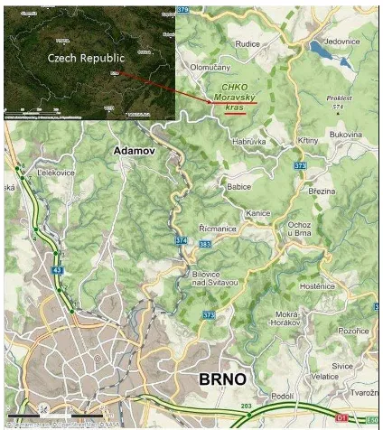
The study area is located in the eastern part of Czech Republic to the north of Brno (Figure 1). The scanning process was performed in two hours, by scanner Riegl VMX – 450 in May 2015. The total length of two covered areas is 3.9 km and 6.1 km respectively, with an average width of 100 m. The two Riegl VQ - 450 laser scanners, the IMU and the GNSS equipment are integrated into measuring head, which was mounted on a roof of a car. The measurement rate of each scanner is 550,000 meas./sec, with a scan rate about 200 profiles/sec. Each scanner provides 360o gapless profile, with high accuracy (8 mm) and precision (5 mm). Тhe first data set (Road 1) contains 8 LAS files (4 from scanner_1 and 4 from scanner_2) with different size from 0.3 to 4.5 gigabytes; the second data set (Road 2) contains 12 LAS files (6 from each scanner) from 0.5 to 3.5 gigabytes.
Figure 1. Study area (Czech - Moravský krás) © Image Copyright 2016, NASA Earth Observatory, Seznam.cz, a.s, OpenStreetMap
2.2 DMR 4G
The Digital Terrain Model of the Czech Republic of the 4th generation (DMR 4G) represents relief of the full Czech Republic in a regular grid of 5 x 5 m. DMR 4G is a product created by The Czech Land Survey Office, in cooperation with the Military Geographical and Hydrometeorological Office from airborne laser scanning data. Laser scanning was performed with LiteMapper 6800 system during 2010 – 2013 years, on an average height 1200 – 1400 m above the terrain in individual blocks. For data filtering and interpolation the software SCOP ++ 5.4 was used. DMR 4G is presented like shaded relief in S-JTSK coordinate system and Height in the Baltic Vertical Datum. The total standard error in bare terrain is near 0.3 m and in forest areas around 1 m. All other information about DMR 4G can be found in Technical Report for DMR 4G in Czech language (Brázdil et al., 2015). In Figure 2, the shaded representation of the DMR 4G is shown for the study area in the Moravian Karst.
Figure 2. Shading of the DMR 4G for the study area in the Moravian Karst (grid size 5 x 5 m), © Data Copyright 2016,
ČÚZK
3. METHODOLOGY
3.1 Algorithms
The proposed methodology for deriving the digital terrain model (DTM) from the MLS data is summarized in the following steps. Each step corresponds to a specific OPALS module and is applied for filtering the terrain points and for interpolating the terrain surface model through the terrain points.
1. Import of the data: opalsImport each LAS file is imported into the opals data manager (odm)
2. Thinning of the points: opalsCell (min Z-value, cellsize – (0.15 x 0.15) m)
3. Import thinned data from both scanners to one data manager: opalsImport all thinned odms into one odm file (note: in next steps, we will process data from scanner_1 and scanner_2 together)
4. Thinning of data from both scanners: opalsCell (second min Z-value, cellsize - 1 m)
5. Preliminary DTM generation based on output from interpolation –robust moving planes)
11. Preliminary DTM generation based on output from step 9: opalsGrid (grid – (0.25 x 0.25) m, interpolation –delaunay)
12. Filling gaps in the DTM: opalsAlgebra
(combination of two grids – outputs from st. 10 & 11)
13. Renewing of the attribute: opalsAddInfo (attribute normalized Z)
14. Robust filtering based on output from step 3 and attribute from step 13: opalsRobfilter (iterations - 100, interpolation plane, normalizedZ < 0.3 m)
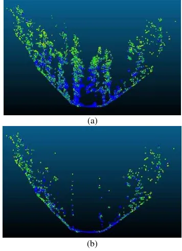
15. Final DTM generation: opalsGrid (robust moving planes, delaunay (triangulation) and moving paraboloid, gridsize – (0.25 x 0.25) m) 1000 [pts/m2]. In some areas on the road or where the roadside trees are very close to the MLS, this number is even higher. The big capacity of data sets makes it hard to handle and process them. For this purpose, we imported files, one by one, to OPALS and applied morphological filtering (steps 1, 2). In each 0.15 x 0.15 m cell we chose the point with smallest Z-value, (b) filtered point cloud with attributes – (0.15 x 0.15) m cell and smallest Z-value from 1 scanner
In steps 4 to 8 and 9 to 13, different combinations of hierarchical interpolations and morphologic filterings are applied to prepare data for robust filtering. Before the first interpolation, we filtered point cloud again. Now, for each (1 x 1) m cell, we chose the second smallest Z-value. The aim of this step is to minimize outliers and make points more homogenous. Then, two interpolation techniques (i.e. robust moving planes and triangulation) are applied with a cell size of 1 x 1 m. For robust moving planes, the number of points used for interpolation was set to 12 with a max. search radius of 2 m. Using the combination of triangulated and robust moving planes grids, we filled gaps in the second one, which were still appearing at trees positions. Then, attribute “normalized Z” can be added to the point cloud by subtracting the preliminary DTM from the z-values. The second interpolation was implemented in the same way, but with other limitations (steps 9 – 13). Now, for each (0.25 x 0.25) m cell we chose the second minimum Z-value and height threshold from (-1 to 0.3 m). This asymmetric height threshold was used to ensure, that all points which are below the fitted plane will be considered. Then, we again interpolated two grids with cell size (0.25 x 0.25) m and renewed our attribute “normalized Z”.
Finally, robust filtering was applied. The parameters are following: search radius 1 m; plane interpolation; a maximum number of iterations is 100; normalized Z below 0.3 m; standard deviation of plane fitting - 0.30. The output from robust filtering is a classified terrain point cloud. Both data sets are processed with the same parameter set. The results of filtering are presented in Table 1.
Table 1. Number of points before and after filtering Captured Data set 1 715,244,450 22,021,269 13,090,319 Data set 2 959,079,445 40,884,798 16,873,583 The International Archives of the Photogrammetry, Remote Sensing and Spatial Information Sciences, Volume XLI-B3, 2016
In Table 1 we can see the number of captured points of an original point cloud, and points before and after robust filtering. Filtered terrain points take in average 2% of measured data set. 98% of other points were filtered based on combinations of hierarchical interpolation and a robust filtering. The average point density of classified terrain points is about 33 [pts/m2].
Finally, extracted terrain points are used for digital terrain generation (step 15). For this purpose, we used three interpolation techniques: robust moving planes, moving paraboloid and triangulation. Each method has its own parameters. For moving planes method, the number of points was set to 30 and maximum search radius 2 m. We tried different combinations of these two parameters. With other settings, the resulted DTM became much smoother or output can be zero. For moving paraboloid method, the number of points was set to 100 and search radius 2 m. For triangulation, we also applied 2 m search radius. Each DTM is generated in (0.25 x 0.25) m grid.
3.2 Comparison with DMR 4G and quality validation
To compare the different data sources (step 16) it has been ensured that the coordinate system are the same. Mobile mapping data and products have ellipsoid Height and UTM 33 coordinates. The Czech Land Survey Office provides data only in S-JTSK/Krovak (East North) – ESPG:102067 coordinate system and Baltic Height. Because DMR 4G has less grid points, we decided to transform it to UTM 33. For this purpose, we used software QGIS. To compute ellipsoid heights for DMR 4G we used quasigeoid CR-2005. To accomplish the comparison, raster images should also have the same grid size.
Before the coordinate transformation, we resampled DMR 4G to grid size (1 x 1) m, and interpolated new DTMs from classified terrain points with grid size (1 x 1) m. Results of the comparison are presented in Table 2, Figure 6 and Appendix.
For the quality check of interpolated DTM, 87 points were measured by a total station on the road area of data set 1 (step 17). The measured profile has a total length about 1 km. For comparison, we chose DTM interpolated by robust moving planes with grid size (0.25 x 0.25) m. The DTM is subtracted from control points. The results are presented in Figure 7.
4. RESULTS
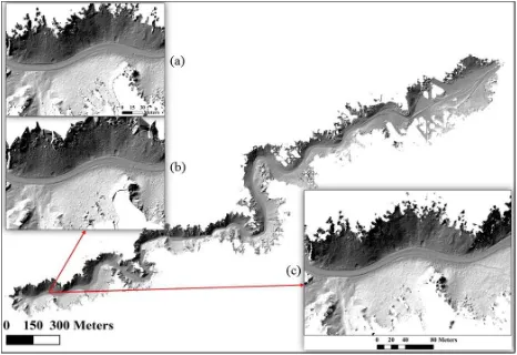
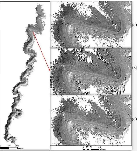
Shadings of the generated DTMs can be seen in Figures 4 and 5. In Figure 4a-c and 5a-c the shadings of DTMs derived from the different interpolation methods are shown.
As we can see in Figure 4b and Figure 5b triangulation interpolation better fill gaps. Robust moving planes method claims to be better for DTM generation in forest areas, during fitting tilted plane, it also detects outliers, which do not take part in interpolation. That is why another solution for DTM generation in our landscape is the combination of robust moving planes and triangulation methods (main images in Figure 4 and Figure 5).
Table 2 presents the height differences between DMR 4G and DTMs interpolated with different interpolation techniques. These differences are summarized from the histograms in
Аppendix.
Figure 4. Shading of the DTM (grid size 0.25 x 0.25 m): main image – road 1 combination of robust moving planes and triangulation; (a) moving paraboloid; (b) triangulation; (c) robust moving planes
Figure 5. Shading of the DTM (grid size 0.25 x 0.25 m): main image – road 2 combination of robust moving planes and triangulation; (a) robust moving planes; (b) triangulation; (c) moving paraboloid
Interpolation method
Da
ta
S
et
1
Heigth Diff. [m]
RobMoving Planes
Moving Paraboloid
Triangulation
Min -35.220 -137.717 -44.066
Max 18.218 127.665 15.909
Mean -0.877 -0.861 -3.143
Median -0.336 -0.318 -0.789
Da
ta
S
et
2
Min -38.187 -122.712 -37.858
Max 19.610 124.879 29.148
Mean -1.415 -1.343 -3.886
Median -0.687 -0.654 -1.490
Table 2. Height difference between DRM 4G and DTMs
The histograms A, B and C show height differences from comparison DMR 4G and data set 1, the histograms D, E, F –
comparison DMR 4G and data set 2. For DTM interpolation new parameters were used: grid size (1 x 1) m, search radius 2 m for triangulation, search radius 1.5 m for moving planes and paraboloid. The number of points used for robust moving planes interpolation are 35 and for moving paraboloid interpolation – 50. The new grid was generated from resampled points from DMR 4G using 50 m search radius and 200 points by robust moving planes interpolation.
As can be seen in Table 2 and in Appendix histograms C and F, the height difference between DMR 4G and triangulated DTM shows the worst results. The average height difference between mentioned grids is more than 3 m when between others it is near 1 m. On the histograms C and F it is shown, that even height differences more than 10 m take almost 15 % in both cases. Triangulation interpolation is not suitable for DTM The International Archives of the Photogrammetry, Remote Sensing and Spatial Information Sciences, Volume XLI-B3, 2016
generation from MLS data. It fills gaps better, but also connects outlier and isolated points that affect the whole grid accuracy.
The average height difference between DMR 4G and robust moving planes DTM is -0.877 m; -1.415 m and moving paraboloid DTM is -0.861 m; -1.343 m. However, for moving paraboloid DTM, the minimum and maximum height differences with DMR 4G are much bigger than from robust moving planes DTM. These results indicate that gross errors are still appearing in generated DTMs and some outlier points take place.
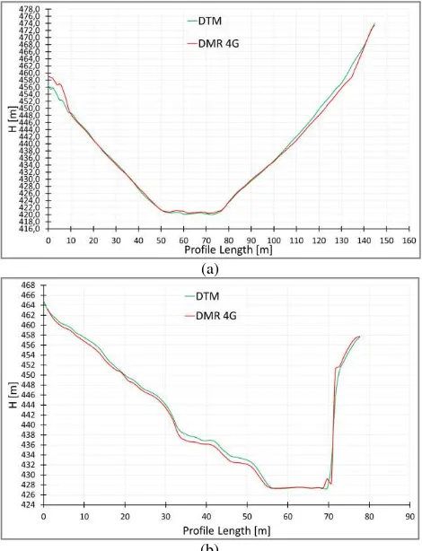
In the histogram A (DMR 4G and robust moving planes DTM comparison) it is shown, that mostly 70% of compared data, has height differences in range from -1 to 1 m. As was mentioned before, the total standard error of DMR 4G in forest areas is 1 m. Let us have a look in Figure 6. It shows the visual profile comparison of DMR 4G (red line) and DTM interpolated by robust moving planes (green line). Axis X is the profile length in meters and axis Y is the height of the terrain. In Figure 6a, it is shown that differences between data are increasing on borders. From 10 to 100 m range the planes are overlapping or difference is less than 1 m, but on borders it is near 2 m or more. Commonly these areas are covered by rocks and are therefore badly reachable for airborne laser scanners especially in dense forests. Histogram D shows the differences between DMR 4G and DTM interpolated by robust moving planes from data set 2. It is shown, that only 50% of the compared data has differences between -1 and 1 m. The area on data set 2 is more steep and rocky than for data set 1. In Figure 6b, it is shown that differences are appearing along all profile, even on a road area.
(a)
(b)
Figure 6. Visual profile comparison of DMR 4G and robust moving planes DTM (a) data set 1 (b) data set 2
Lastly, the height differences between the reference points and the derived DTM are shown in the histogram in Figure 7. The average height difference is 0.095 m, the maximum is near 0.20 m and minimum 0.02 m. In the histogram it is shown, that all values are negative, this means that reference heights are lower than DTM heights. This can be impacted by different measurement equipment (total station vs MLS), their accuracy, weather conditions and placement of satellites, etc. Also, this height shift can be explained by the quality of GNSS signal. For good results we need at least 4 satellites, however in such forest areas, this requirement cannot always be observed. These results show the high quality of derived DTM. However, other areas should also be explored.
Figure 7. Height difference between control points and DTM robust moving planes
5. CONCLUSIONS
In this work, we have presented a fully automatic algorithm for generation of Digital Terrain Model from several Mobile Laser Scanning data sets captured in the neighbourhood of a forest road.
Firstly, MLS data sets are processed and filtered using hierarchical interpolation and a robust filtering. Filtered terrain points take in average only 2% of the data set. After extraction of ground points, different interpolation methods are applied for DTM generation. The grid size of interpolated DTMs is (0.25 x 0.25) m. The average vertical accuracy is 0.10 m, checked by geodetic measurements of 87 points on the 1 km long road area. The derived DTM can be used for analysing terrain changes and morphological structures, modelling of water flows and exploring geological features. We have compared generated DTMs with DMR 4G, which has been generated from airborne laser scanning data. The biggest height difference occurs in rock places, which are difficult to reach, and which are often affected by occlusions.
In future work, we will have to consider more filtering algorithms or their combination, to improve a better quality of terrain extraction from MLS data in rock areas to eliminate outlier, non-terrain and other classification errors that have a big influence on resulting products.
ACKNOWLEDGEMENTS
This work is partly founded from the European Community’s Seventh Framework Programme (FP7/2007–2013) under grant agreement No. 606971, the Advanced_SAR project. The authors would like to thank AdMaS centre (BUT Brno) for providing MLS data and Research Group of Photogrammetry (TU Wien) for collaboration and assistance.
REFERENCES
Bitenc, M., Lindenbergh, R., Khoshelham, K., Van Waarden, A. P., 2011. Evaluation of a LiDAR land-based mobile mapping system for monitoring sandy coasts. Remote Sensing, 3(7), pp.
Gorte, B., Elberink, S. O., Sirmacek, B., Wang, J., 2015. IQPC 2015 track: Tree separation and classification in mobile mapping lidar data. In: The International Archives of Photogrammetry, Remote Sensing and Spatial Information Sciences, 40(3), pp. 607-612.
Jaakkola, A., Hyyppä, J., Hyyppä, H., Kukko, A., 2008. Retrieval algorithms for road surface modelling using laser-based mobile mapping. Sensors, 8(9), pp. 5238-5249.
Kraus, K. and Pfeifer, N., 1998. Determination of terrain models in wooded areas with airborne laser scanner data. ISPRS Journal of Photogrammetry and Remote Sensing, 53(4), pp. 193-203.
Lehtomaki, M., Jaakkola, A., Hyyppa, J., Lampinen, J., Kaartinen, H., Kukko, A., Puttonen, E., Hyyppa, H., 2016. Object Classification and Recognition From Mobile Laser Scanning Point Clouds in a Road Environment. In: IEEE Transactions on Geoscience and Remote Sensing, vol. 54, no. 2, pp. 1226-1239.
Lindenbergh, R. C., Berthold, D., Sirmacek, B., Herrero-Huerta, M., Wang, J., Ebersbach, D., 2015. Automated large scale parameter extraction of road-side trees sampled by a laser mobile mapping system. In: The International Archives of Photogrammetry, Remote Sensing and Spatial Information Sciences, 40(3), pp. 589-594.
Mandlburger, G., Otepka, J., Karel, W., Wagner, W., Pfeifer, N., 2009. Orientation and processing of airborne laser scanning data (OPALS)—Concept and first results of a comprehensive ALS software. In: Proceedings of the ISPRS Workshop Laserscanning, Vol. 9, pp. 55-60.
Nurunnabi, A., West, G., & Belton, D. 2013. Robust locally weighted regression for ground surface extraction in mobile laser scanning 3D data. In: ISPRS Annals of Photogrammetry, Remote Sensing and Spatial Information Sciences, 1(2), pp. 217-222.
Otepka, J., Mandlburger, G., Karel, W., 2012. The OPALS Data Manager—Efficient Data Management for Processing Large Airborne Laser Scanning Projects. In: Proceedings of the ISPRS Annals of the Photogrammetry, Vol. 1-3, pp. 153-159.
Pfeifer, N., Kraus, K., Köstli, A., 1999. Restitution of airborne laser scanner data in wooded areas. GIS-HEIDELBERG-, 12, Recognizing basic structures from mobile laser scanning data for road inventory studies. ISPRS Journal of Photogrammetry and Remote Sensing, 66(6), pp. S28-S39.
Sithole, G., and Vosselman, G., 2004. Experimental comparison of filter algorithms for bare-Earth extraction from airborne laser scanning point clouds. ISPRS Journal of Photogrammetry and Remote Sensing, 59(1), pp. 85-101.
Vallet, B. and Papelard, J. P., 2015. Road orthophoto/DTM generation from mobile laser scanning. In: International Annals of Photogrammetry Remote Sensing and Spatial Information Sciences, 3, W5, pp. 377-384.
Wang, J., Gonzalez-Jorge, H., Lindenbergh, R., Arias-Sanchez, P., Menenti, M., 2014. Geometric road runoff estimation from laser mobile mapping data. In: ISPRS Annals of the Photogrammetry, Remote Sensing and Spatial Information Sciences, 2(5), pp. 385-391.
APPENDIX