A NEW DIGITAL IMAGE CORRELATION SOFTWARE FOR DISPLACEMENTS FIELD
MEASUREMENT IN STRUCTURAL APPLICATIONS
R. Ravanellia∗, A. Nascettia, M. Di Ritaa, V. Bellonia, D. Matteib, N. Nistic´ob, M. Crespia
a
Geodesy and Geomatics Division, DICEA - University of Rome “La Sapienza”, Rome, Italy <roberta.ravanelli, martina.dirita, andrea.nascetti, mattia.crespi>@uniroma1.it b
Department of Structural and Geotechnical Engineering - University of Rome “La Sapienza”, Rome, Italy <nicola.nistico>@uniroma1.it
Commission IV WG IV/4
KEY WORDS:Digital Image Correlation (DIC), Free and Open Souce Software, Close range photogrammetry, Structural Applications
ABSTRACT:
Recently, there has been a growing interest in studying non-contact techniques for strain and displacement measurement. Within photogrammetry, Digital Image Correlation (DIC) has received particular attention thanks to the recent advances in the field of low-cost, high resolution digital cameras, computer power and memory storage. DIC is indeed an optical technique able to measure full field displacements and strain by comparing digital images of the surface of a material sample at different stages of deformation and thus can play a major role in structural monitoring applications.
For all these reasons, a free and open source 2D DIC software, named py2DIC, was developed at the Geodesy and Geomatics Division of DICEA, University of Rome ”La Sapienza”. Completely written in python, the software is based on the template matching method and computes the displacement and strain fields. The potentialities of Py2DIC were evaluated by processing the images captured during a tensile test performed in the Lab of Structural Engineering, where three different Glass Fiber Reinforced Polymer samples were subjected to a controlled tension by means of a universal testing machine.
The results, compared with the values independently measured by several strain gauges fixed on the samples, demonstrate the possibility to successfully characterize the deformation mechanism of the investigated material. Py2DIC is indeed able to highlight displacements at few microns level, in reasonable agreement with the reference, both in terms of displacements (again, at few microns in the average) and Poisson’s module.
1. INTRODUCTION
Strain and displacement are essential parameters in structural en-gineering. Nevertheless, their measurement is difficult outside laboratory conditions because of the complex setup that the tra-ditional techniques need (e.g. strain gauges). For this reason, re-cently, there has been a growing interest in studying non-contact measurement techniques, which do not require the use of dedi-cated devices.
In particular, the photogrammetric technique has received atten-tion for this kind of applicaatten-tions, thanks to its ability to suc-ceed in achieving full field measurements through images anal-ysis, and its robustness to work in testing environments. As a matter of fact, photogrammetry can be used to extract geometry, displacement, strain and deformation velocity of different ma-terials or structures subjected to incremental loads using digital images. Furthermore, due to the advances in the field of low-cost, high resolution digital cameras, computer power and mem-ory storage, photogrammetric applications widened also to struc-tural, mechanical and civil engineering.
Digital Image Correlation (DIC) is the term used in structural en-gineering applications to refer to the well-known template match-ing method, generally used in photogrammetry and computer vi-sion to retrieve homologous points. DIC is a technique used to study structural phenomena and perform strain and displacement measurements. It compares a series of images of a sample at different stages of deformation, tracks pixels movement in the region of interest (ROI) and calculates displacement and strain
∗Corresponding author
by tracking (or matching) the same points between the recorded images using matching algorithms (McCormick and Lord, 2010). DIC can be used in 2D and 3D analysis, being the first one limited to in-plane deformation measurement of the planar object sur-face: if the test object is a curved surface, or if a 3D deformation occurs after loading, the 2D DIC method is no longer applicable and a 3D DIC based on the principle of binocular stereovision is needed (Pan et al., 2009). In that case, two fixed cameras are needed, while in 2D DIC only one is used.
Nowadays, there are various commercial software available in the market based on 2D DIC to evaluate strain and displacement fields. However, the limitations of using commercial software are their inherent costs, and the restrictions imposed to users because no customizations of the source code, to better fit their require-ments, are allowed. Alternatively, an open source, user friendly software can remarkably reduce costs and can be tailored to user needs.
For this reason, a new, free and open source 2D DIC software (FOSS4G), named py2DIC, was developed at the Geodesy and Geomatics Division, University of Rome ”La Sapienza”. It has been developed in Python programming language and the source code is freely available athttps://github.com/Geod-Geom/ py2DIC. Some other free and an open source software for DIC analysis are available, but generally in Matlab language (e.g. (Jones et al., 2014)), for which a license is necessary.
obtained results. In the end, in Section 5, some conclusions are drawn and future prospects are outlined.
2. PY2DIC
The py2DIC software was developed at the Geodesy and Geomat-ics Division of DICEA, University of Rome ”La Sapienza”. Free and open source, the software is based on the template match-ing method, a well-known technique for matchmatch-ing patterns based upon cross-correlation, and returns the displacement and strain fields by comparing two or more images of the sample acquired at different stages of deformation.
The software, completely written in Python, is provided with a Graphical User Interface (GUI), and it leverages the potential-ities of OpenCV (Bradski and Kaehler, 2008), an open source computer vision and machine learning software library.
The template matching technique implemented in the 2D DIC software consists of several steps. First of all, the region of in-terest is divided into a grid of uniformly spaced points; then, the normalized cross-correlation index is calculated by convolving a portion of the reference image (thereference template) with the corresponding larger subset (thesearch window) in the search im-age, as shown in Figure 1. The selected displacement(u, v)is the one which maximizes the value of the correlation coefficient.
Figure 1: Scheme of the image pairs together with the reference template, the central pixel and the search window.
Specifically, it is necessary to consider the pixelp(x, y)in the reference image located at the central point of the template and to open the search window in the search image exactly around the same pixel. In fact, assuming that the camera remains fixed dur-ing the acquisition of the images, the reference system of the two images can be considered the same. Furthermore, if the size of the reference template is(w×w), the size of the search window
must be(w+d)×(w+b), wherewis the template width and dandbare the edge along thexandydirection respectively. To obtain a good matching, it is important to choose an edge which is greater than the maximum displacement expected, otherwise the test block on the search image, which corresponds to the tem-plate of the reference image, will not be found in the search area. The core of the procedure is performed by using the OpenCV functioncv2.matchTemplatewith the FNCC (Fast Normalized Cross-Correlation) correlation criterion.
Finally, by sliding the reference template all over the search im-age, the displacements are computed for each node of the grid, as shown in Figure 6a. It is important to underline that the whole set of the template central points constitute the grid, whose dimen-sions depend on the size in pixels of the reference template.
Concerning the strains, they are computed through a numerical differentiation process of the estimated displacements:
ǫx=
whereǫx and ǫy are the horizontal and vertical strains, andu
andvdenote the x-directional displacement and the y-directional displacement; the centered difference approximation is used, by replacing each derivative by a finite difference:
ǫx=
where:ǫxandǫyare the horizontal and vertical strains;ui+1and ui−1are the the x-directional displacements at i+1 and i-1 points; vj+1andvj−1are the y-directional displacements at j+1 and j-1 points;∆xand∆yare the grid spacing.
2.1 The graphical user interface
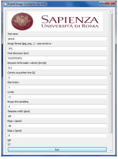
The GUI, shown in Figure 2, is developed with PyQt4 and allows to set easily the parameters required for the data processing. First of all, it is necessary to specify the name of the folder containing the images to be processed and their format.
Figure 2: The graphical user interface.
using the ruler, it is simple to obtain the pixel dimension in metric units.
The imposed deformation velocity refers to the velocity imposed by the tensile testing machine to deform the sample. The cam-era acquisition time is the time period of acquisition between two images: it represents the images time sampling and for our tests it was equal to 5 seconds. The start index is the parameter used to select the first image that the software analyses and the levels refer to the number of images which are used to calculate dis-placements.
The image time sampling is used to select some images and re-duce the computational time. The last three parameters are the template and the edge along x and y direction and they are ex-pressed in pixels. The template size must be defined carefully: if the template is too small the noise increases whereas if it is too big there is a risk of losing displacements.
Furthermore, an interface was implemented to select the area of interest on the sample images before starting the processing. Once the image is opened, a yellow rectangle is drawn on the image through mouse click events to indicate the outline of the selection, as shown in Figure 9. Finally, after setting the required parameters and pressing the Run button, the software begins to process the images.
2.2 The software outcomes
As already described before, the 2D DIC software computes dis-placements(u, v)and strains (∂u
∂x, ∂v
∂y) by comparing two or more
images of the sample acquired at different stages of deformation.
The software allows to perform the analysis in several steps: the results are the accumulated displacements and strains for each step of calculation and are reported into text files for each pair of processed images. The first file contains the coordinates of the grid point, the displacements alongxandydirection and the length of the displacement vector for each point of the grid. The other files show the values of displacements and strains for each point of the grid separately.
Furthermore, the displacement and strain maps, the displacement quiver plot and the displacement plot related to the central section of the sample are shown at the end of the process and saved in the output folder (Figure 4a, Figure 4b, Figure 5a, Figure 5b, Figure 6a, Figure 6b).
Finally, it is also possible to create animated GIFs of the output images selecting the option by a check mark in the graphical user interface as shown in Figure 2.
3. THE EXPERIMETAL SETUP
Some experiments were conducted in order to investigate the po-tentialities of the developed software. In particular, the images acquired during a tensile test performed in the Lab of Structural Engineering were processed (Mattei, 2017), (Belloni, 2017).
Specifically, Glass Fiber Reinforced Polymer samples were sub-jected to a controlled tension by means of a universal testing ma-chine (see Figure 3). The tests were carried out by placing the sample in the grips of the testing machine and slowly extending it until failure. During the process, the elongation of the gauge section was recorded against the applied force and the deforma-tion rate was imposed equal to 0.5 mm per minute.
Figure 3: The experimental setup: the testing machine and the camera.
The Canon EOS 1200D camera, used to record the images, was connected to a standard laptop and placed near the sample, fixed on a metallic bar (Figure 3) in order to avoid vibrations during the loading tests. The images were captured through the EOS Digital Solutions Disk Software with a time sampling of one acquisition every 5 seconds and a resolution of 5184×3456 pixels.
Finally, several strain gauges were fixed on the sample to inde-pendently measure the strain value throughout the loading tests: they served as reference to evaluate the results obtained with the developed software. Here we just recall that a strain gauge is a sensor whose electrical resistance varies with the applied strain; measuring the variation of electrical resistance of the strain gauge, the amount of induced strain can be inferred.
4. RESULTS
The images acquired during the tests were processed through the developed software and the results were compared with the dis-placements inferred from the strain values measured by means of the strain gauges. Three samples, cut from a GFRP beam along different fiber orientations, were used during the tests, as shown in Figure 7 and Table 1.
Sample n. Orientation Width Height Thickness
[◦] [mm] [mm] [mm]
1 90 30 120 8
2 0 30 124 8
3 45 30 164 8
Table 1: Features of the three samples.
For the first test, four strain gauges were installed on the sample with 90◦fiber orientation (see Figure 8). One was placed
(a) (b)
Figure 4: (a) The horizontal and (b) vertical displacements.
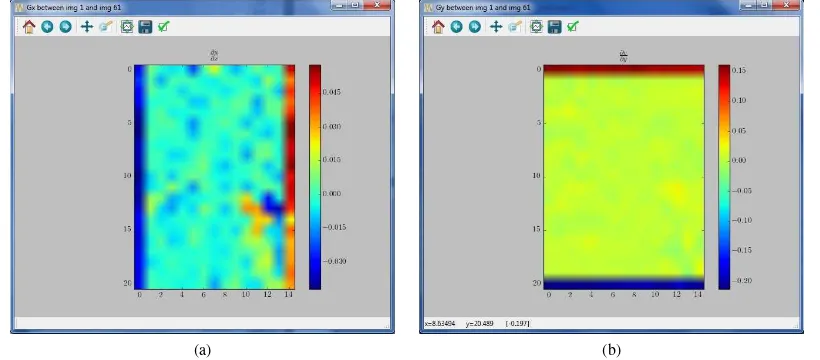
(a) (b)
Figure 5: (a) The horizontal and (b) vertical strains.
(a) (b)
Figure 6: (a) Quiver plot of the computed displacements and (b) displacement plot of the sample central section.
fixed on the opposite side with the same disposition. Finally, the last two strain gauges were located vertically on the lateral sides in order to measure the vertical strain.
Figure 7: The three samples with different fiber orientations.
Figure 8: The strain gauges disposition on the 90◦fiber
orienta-tion sample.
was placed on the lateral side of the sample, the vertical displace-ments were computed through the DIC software considering the right side of the region facing the camera (see Figure 9), very near to the area effectively occupied by the strain gauge.
Figure 9: In yellow the selected area for vertical dispalcements.
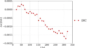
In particular, the software computed the displacements for ev-ery node of the grid. Then, exclusively the displacements of the points located near the extremities of the strain gauge were con-sidered for the subsequent analysis: they were spatially averaged, producing thus two values, one representative for the upper part of the strain gauge and one representative for the lower part. In this way, it was possible to compare the difference between these two DIC displacements with the strain measured by the strain gauge, multiplied by the gauge length. This calculation was per-formed at different time steps and the vertical displacements∆v versus time are plotted in Figure 10.
It can be noticed that the DIC results well follow the trend of the displacements inferred by the strain gauge measurements; the RMSE of the DIC computed displacements with respect to the strain gauge reference is of the order of some microns. Anyway, in this first test, it was not possible to compare the DIC results neither with the strain gauge n. 3, since the wires covered the sample on the area of interest, representing a source of error, nei-ther with the strain gauge n. 2, since the horizontal displacements were too small for the ground sampling distance used (the camera was too far from the sample).
During the second test, the 0◦fiber orientation sample was used.
The sample was prepared fixing three strain gauges: two of them
Figure 10: Comparison between the vertical displacements ob-tained by the DIC method and the strain gauges measurements for sample n. 1.
were installed vertically on the lateral sides to measure the verti-cal strain whereas the last one (the strain gauge n. 2) was placed horizontally on the side facing the camera being in such way able to measure the horizontal strain. For this second test, both ver-tical and horizontal displacements were calculated with the DIC software.
Concerning the horizontal displacements, the strain gauge n. 2 was considered as reference. Also in this second test, the DIC displacements were averaged spatially on the grid points near the two extremities (left and right) of the strain gauge, respectively. Then the difference between these two averaged displacements was computed twice: one at the bottom end part and one at the top end part of the strain gauge, since the wires covered the cen-tral section. Therefore, the mean between these two values was compared with the displacements inferred by the strain gauge at different time steps, as Figure 11 shows: the DIC trend well fol-lows the reference in this test, too.
Figure 11: Comparison between the horizontal displacements obtained by the DIC software and the strain gauges measurements for sample n. 2.
Regarding the vertical displacements, the same approach adopted in the first test was used, this time for both the sides of the sam-ple. The displacements∆vversus time are thus plotted in Figure 12: the displacements obtained through the developed software are slightly different from those observed by the strain gauges, displaying a bias in the trend. This behaviour is probably due to the fact that eccentricity occurred during the test. Furthermore, it is important to remember that the DIC method was applied on a region of the sample that did not coincide exactly with the areas on which the strain gauges were fixed.
Finally, the Poisson’s ratio was calculated at different time steps with the following well known equation:
ν=−ǫx
ǫy
Figure 12: Comparison between the vertical displacements ob-tained by the DIC method and the strain gauges measurements for sample n. 2.
whereǫxandǫydenote the horizontal strain and vertical strain,
respectively. The computed Poisson’s ratio trend is plotted in Figure 13, together with the Poisson’s ratio related to the strain gauges measurements; the mean values of Poisson’s ratio, com-puted considering exclusively the stable trend, are reported in Ta-ble 2.
Figure 13: Comparison between the Poisson’s ratio obtained by the DIC method and the strain gauges measurements for sample n. 2.
DIC Strain gauges ν 0.21 0.27
Table 2: Poisson’s ratio comparison for test n. 2.
For the third test, three strain gauges were installed on the sample with 45◦fiber orientation, as shown in Figure 14. Two of them
were fixed vertically on the lateral sides whereas the other was installed on the side facing the camera with a 45◦orientation.
Figure 14: The strain gauges disposition on the 45◦fiber
orien-tation sample.
As in the previous case, the vertical and horizontal displacements were calculated at different time steps and are reported in Figure 15 and Figure 16, respectively.
Figure 15: Comparison between the vertical displacements ob-tained by the DIC method and the strain gauges measurements for sample n. 3.
Figure 16: Horizontal displacements obtained by the DIC method for sample n. 3.
As regards the horizontal displacements, it was not possible to make a comparison since no horizontal strain gauge was fixed on the sample during this test. On the other hand, the computed vertical displacements, once again in accordance with the values measured by the strain gauges, confirm the good performances of the developed software. Also for this last test, the Poisson’s ratio was calculated at different time steps, as shown in Figure 17, presenting a mean value of 0.37.
Figure 17: Poisson’s ratio trend for sample n. 3.
Anyway, since the strain gauges n. 2 was installed with a 45◦
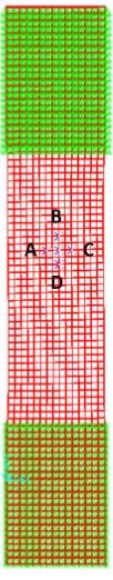
orientation, the computed Poisson’s ratio value was compared with the one obtained through the Finite Element Method model (FEM) implemented within SAP2000 (Computers and Structures Inc, 2017) software (Mattei, 2017). The modelled sample is il-lustrated in Figure 18, where the four different points considered to evaluate the Poisson’s ratio are reported, too.
Starting from the displacement values of these points, thex−
(horizontal) andy−(vertical) directional strain were calculated,
Figure 18: The FEM model.
DIC SAP2000 model
ν 0.37 0.4
Table 3: Poisson’s ratio comparison for the test n. 3.
5. CONCLUSIONS
Py2DIC, a new, free and open source 2D Digital Image Correla-tion software was developed at the Geodesy and Geomatics Divi-sion of DICEA - University of Rome ”La Sapienza”.
The potentialities of the developed software were investigated by processing the images acquired during a tensile test performed in the Lab of Structural Engineering, where three different Glass Fiber Reinforced Polymer samples were subjected to a controlled tension by means of a universal testing machine.
The obtained results were compared with the values indepen-dently measured by several strain gauges fixed on the samples, and demonstrate the possibility to successfully characterize the deformation mechanism of a GFRP material subjected to me-chanical loading.
The implemented DIC method is indeed able to highlight dis-placements at few microns level, in reasonable agreement with the reference, both in terms of displacements (again, at few mi-crons in the average) and Poisson’s module.
Finally, as a future work, it would be worth using a digital ac-quisition system characterized by a higher frame rate, in order to study transient phenomena such as fractures, and implement-ing a DIC stereo approach in order to characterize also the 3D deformations which can occur during the loading tests.
ACKNOWLEDGEMENTS
The authors are indebted with the Lab of Structural Engineering of University of Rome ”La Sapienza” for the assistance during
the tensile experiments.
REFERENCES
Belloni, V., 2017. A new Digital Image Correlation software for displacements field measurement in structural applications. M.S. Thesis, University of Rome ”La Sapienza”, Faculty of Civil and Industrial Engineering.
Bradski, G. and Kaehler, A., 2008. Learning OpenCV: Computer vision with the OpenCV library. O’Reilly Media, Inc.
Computers and Structures Inc, 2017. https://www. csiamerica.com/products/sap2000.
Jones, E. M. C., Silberstein, M. N., White, S. R. and Sottos, N. R., 2014. In situ measurements of strains in composite battery elec-trodes during electrochemical cycling. Experimental Mechanics 54(6), pp. 971–985.
Mattei, D., 2017. Fiber reinforced polymer structural elements: analysis and modeling. M.S. Thesis, University of Rome ”La Sapienza”, Faculty of Civil and Industrial Engineering.
McCormick, N. and Lord, J., 2010. Digital image correlation. Materials Today 13(12), pp. 52 – 54.